This is meant as a beginning guide to Bezier surfaces and some ways to implement them in practical code. This isn't meant as a thorough exploration of the mathematics, but as a jump-off point. I'm sure others here know more than I do, but I'd like to introduce some things here that can be helpful to those who want to delve into this topic. If you're not familiar with the Bezier formulation for curves, please read "
The Practical Guide to Bezier Curves" article first.
The Bernstein Basis Functions
The quickest way to do a single evaluation of a point on the Bezier surface is to evaluate the Bernstein basis functions directly. Recall the formal Bernstein basis function form:
\[
B(t) = \binom{n}{i} (1-t)^{n-i} t^i
\]
Naive evaluation will take a long time computationally, especially considering that the binomial term is often expressed in terms of factorials. Let's see if we can't use a trick or two to cut this down. Bernstein basis functions have some unique properties. Leveraging these properties will help us do more quick evaluations. Here's a short list of the properties of Bernstein basis functions:
- Nonnegativity: \(B_{i,n}(u) \geq 0 \,\, \forall i,n \, \text{and} \, 0 \leq u \leq 1\)
- Partition of Unity: \(\sum \limits_{i=0}^n B_{i,n}(u) = 1\)
- Endpoint Interpolation: \(B_{0,n}(0) = B_{n,n}(1) = 1\)
- Single Maximum: \(\text{max} \left ( B_{i,n}(u) \right ) \, \text{at} \, u=\frac{i}{n} \)
- Recursive: \( B_{i,n}(u) = (1-u)B_{i,n-1}(u) + uB_{i-1,n-1}(u),\,\,B_{i,n}(u) = 0 \, \text{if} \, i \le 0 \, \text{or} \, i \ge n \)
- Derivative: \( \prime{B}_{i,n}(u) = n \left ( B_{i-1,n-1}(u) - B_{i,n-1}(u) \right ), \, B_{-1,n-1}(u) = B_{n,n-1}(u) = 0 \)
The recursive property allows us to construct higher order basis functions from lower order ones. From the Bernstein basis definition, we know that \(B_{0,0} = 1]), so we can set up a loop to construct the basis functions from degree-0 to degree-n. For Bernstein polynomials of degree n, we will have (n+1) basis functions at the end. Code in C# to compute the Bernstein basis functions would look like this:
public double[] GetBasisFunctions(int n, double t)
{
    double[] F = new double[n+1];
	F[0] = 1;
	double u = 1.0 - t;

	for(int j = 1; j <= n; j++)
	{
		for(int i = j; i >= 0; i--)
		{
			double lp = (i > n ? 0 : u * F);
			double rp = (i - 1 < 0 ? 0 : t * F[i-1]);
			F = lp + rp;
		}
	}
	return F;
}
Matrix Form and Bezier Curves
Bernstein basis forms are good for evaluating single points, but what if you want to evaluate a lot of points all at once, like a grid? Let's look at the matrix formulation of a Bezier curve. This is actually a good starting point because we can expand this to work for surfaces. To "derive" the formulas, let's take the expansion of a cubic (degree-3) Bezier curve:
\[ B(t) = \binom{3}{0}P_0(1-t)^3 + \binom{3}{1}P_1t(1-t)^2 + \binom{3}{2}P_2(1-t)t^2 + \binom{3}{3}P_3t^3 \]
This isn't anything you haven't seen before. But, we can convert this into an equivalent matrix form:
\[
B(t)=
\begin{bmatrix} P_0 & P_1 & P_2 & P_3 \\ \end{bmatrix}
\begin{bmatrix} \binom{3}{0}(1-t)^3 \\ \binom{3}{1}t(1-t)^2 \\ \binom{3}{2}t^2(1-t) \\ \binom{3}{3}t^3 \\ \end{bmatrix}
\]
If you're not comfortable with this, multiply it out and check the result. This is a nice math trick, but there is no significant advantage to this, is there? Not yet, but there can be if we notice that we've separated the equation so that the parametric variable
t appears in only the right column vector matrix. It's still in terms of the Bernstein basis functions, so it doesn't help us too much yet. Now, let's expand the basis functions:
\[
B(t)=
\begin{bmatrix} P_0 & P_1 & P_2 & P_3 \\ \end{bmatrix}
\begin{bmatrix} \binom{3}{0}(-t^3+3t^2-3t+1) \\ \binom{3}{1}(t^3-2t^2+t) \\ \binom{3}{2}(-t^3+t^2) \\ \binom{3}{3}t^3 \\ \end{bmatrix}
\]
This looks like it's getting complicated. Well, it is and it isn't. If we split this column vector up into a couple of more matrices (I promise we're at the end of this), we can get something more simplified:
\[
B(t)=
\begin{bmatrix} P_0 & P_1 & P_2 & P_3 \\ \end{bmatrix}
\begin{bmatrix}
\binom{3}{0}(-1) & \binom{3}{0}(3) & \binom{3}{0}(-3) & \binom{3}{0}(1) \\
\binom{3}{1}(1) & \binom{3}{1}(-2) & \binom{3}{1}(1) & 0 \\
\binom{3}{2}(-1) & \binom{3}{2}(1) & 0 & 0 \\
\binom{3}{3}(1) & 0 & 0 & 0 \\
\end{bmatrix}
\begin{bmatrix} t^3 \\ t^2 \\ t \\ 1 \end{bmatrix}
\]
Isn't that beautiful? We've reduced the Bezier curve to 3 matrices and separated out the parametric variable into a simple column vector. If we want to evaluate the whole curve efficiently, we can simply multiply the first 2 matrices, and multiply it by the column vector for every parameter value. The simple form for the triangular part of the matrix holding the binomial coefficient can be calculated with this formula:
\[ M(i,j) = \begin{cases}
\binom{n}{i} \binom{n-i}{j} (-1)^{n+i-j}; & 0 \le i \le n, \, 0 \le j \le n-i \\
0, & \text{otherwise} \\
\end{cases}
\]
Uses for Matrix Form
Now, this form isn't just elegant, it's useful. For what? Well...for a couple things. First off, we can get derivative information here really easily. The derivative of the curve is dB/dt, so by differentiating the parametric terms, we can calculate the derivative. And since the parametric terms are all collected in a column vector, that's the only matrix we need to change! To calculate the derivative in the example, it's just:
\[
B'(t)=
\begin{bmatrix} P_0 & P_1 & P_2 & P_3 \\ \end{bmatrix}
\begin{bmatrix}
\binom{3}{0}(-1) & \binom{3}{0}(3) & \binom{3}{0}(-3) & \binom{3}{0}(1) \\
\binom{3}{1}(1) & \binom{3}{1}(-2) & \binom{3}{1}(1) & 0 \\
\binom{3}{2}(-1) & \binom{3}{2}(1) & 0 & 0 \\
\binom{3}{3}(1) & 0 & 0 & 0 \\
\end{bmatrix}
\begin{bmatrix} 3t^2 \\ 2t \\ 1 \\ 0 \end{bmatrix}
\]
Now, you might be saying, "Hey, this form is way harder than the control point subtraction method of finding the derivative of the curve!" Well, to that I say....yeah, it is...for curves at least. When we discuss surfaces, you'll thank me for this. I promise.
The other thing this form allows us to do is to express surfaces very simply.
Bezier Surfaces
Background
Disclaimer: There is a lot of information on surfaces that I could have given here, but I've been chided about going too far into numerical analysis with this stuff, so I've tried to cut down on the un-game-related info. If I've been too light on some stuff here, let me know in the comments and I'll try to add it later.
In math jargon, a Bezier surface patch is called a tensor-product surface because it is the product of pairs of univariate blending functions, in this case, the Bernstein basis functions. This might be alien speak to you, but don't worry, you won't have to understand it. Really, this means a couple of things:
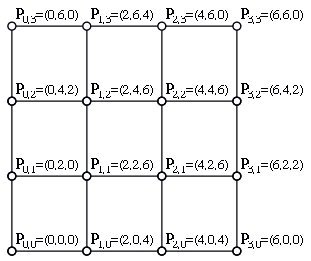
- This surface is formed from a rectangular grid of control points.
- This surface is a function of two independent variables.
- This surface depends on two separate blending functions.
A condensed form of the surface equation looks like this:
\[ S(u,v) = \sum_{j=0}^m \sum_{i=0}^m P_{ij}B_i^m(u)B_j^n(v) \]
Here, you can see how similar this is to a Bezier curve. The main differences are the presence of another variable and thus another blending function, and the control points form a grid or net. To evaluate a point on the surface, simply plug in the values for
u and
v into the Bernstein blending functions, multiply that by the all the control points in the grid and sum them all up. It's really just like a Bezier curve in that respect.
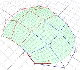
The only thing we have to understand now is that there are 2 parameter coordinates for each point on the surface,
u and
v. I refer to these u- and v- "directions" to describe the surfaces because the control points can be in 2D or 3D, so the only way to describe things are in terms of the parameters.
Bernstein Basis Form
For this method, we can evaluate the Bernstein basis functions for the u- and v-parameters. Then, we just have to multiply the correct evaluated Bernstein basis functions together with the control point, just like in the formal definition.
As mentioned before, this method is fine for evaluating a few points on the surface, but it's not optimal for quick evaluation of the entire surface. This is because we have to compute new Bernstein basis function sets for each (u,v) points. For large sets of evaluation points, the matrix method is better.
Matrix Form
To make it look even more like the Bezier curve form, we can convert this to matrix form using the technique as explained above. The resulting form for a bicubic surface patch (cubic in both u- and v-parameter directions) is as follows:
\[
S(u,v) =
\begin{bmatrix} v^3 & v^2 & v & 1 \\ \end{bmatrix}
\begin{bmatrix}
\binom{3}{0}(-1) & \binom{3}{0}(3) & \binom{3}{0}(-3) & \binom{3}{0}(1) \\
\binom{3}{1}(1) & \binom{3}{1}(-2) & \binom{3}{1}(1) & 0 \\
\binom{3}{2}(-1) & \binom{3}{2}(1) & 0 & 0 \\
\binom{3}{3}(1) & 0 & 0 & 0 \\
\end{bmatrix}
\begin{bmatrix}
P_{00} & P_{01} & P_{02} & P_{03} \\
P_{10} & P_{11} & P_{12} & P_{13} \\
P_{20} & P_{21} & P_{22} & P_{23} \\
P_{30} & P_{31} & P_{32} & P_{33} \\
\end{bmatrix}
\begin{bmatrix}
\binom{3}{0}(-1) & \binom{3}{0}(3) & \binom{3}{0}(-3) & \binom{3}{0}(1) \\
\binom{3}{1}(1) & \binom{3}{1}(-2) & \binom{3}{1}(1) & 0 \\
\binom{3}{2}(-1) & \binom{3}{2}(1) & 0 & 0 \\
\binom{3}{3}(1) & 0 & 0 & 0 \\
\end{bmatrix}
\begin{bmatrix} u^3 \\ u^2 \\ u \\ 1 \end{bmatrix}
\]
Again, if you're not comfortable, multiply it out and check this for yourself. As you can see, in this form the surface really doesn't look too much different than the curve! Sure, there's another set of matrices on the left side and the center matrix is now not a vector, but that's really it. A simplified form of this is:
\[ S(u,v) = \mathbf{v}\mathbf{M_v}\mathbf{P}\mathbf{M_u}\mathbf{u} \]
The Mu and Mv matrices are constructed with the same formula as above. Notice, however, that the patch doesn't need to be bicubic; each direction can be a different degree. If in the u-direction the patch is quadratic (degree-2) and quartic (degree-4) in the v-direction, it only really changes the size of the matrices, not the formulation. In this example, the Mu matrix would be 3x3, the u-parameter matrix would be 3x1, the Mv matrix would be 5x5, the v-parameter matrix would be 1x5, and the control point grid matrix would be 5x3. Thus, the multiplication would produce a 1x1 matrix, the evaluated point on the surface.
If we want to evaluate the surface quickly, we can precompute the multiplication of the center 3 matrices (Mv*P*Mu) and then change the u- and v-parameter matrices for every value and then multiply to get the points on the surface:
\[ S(u,v) =
\begin{bmatrix} v^3 & v^2 & v & 1 \\ \end{bmatrix}
\mathbf{M_vPM_u}
\begin{bmatrix} u^3 \\ u^2 \\ u \\ 1 \end{bmatrix}
\]
Derivatives and Surface Normals
This is all fine and good to get the surface points, but when we render surfaces, we need surface normals! Thus, we'll need to compute derivatives. Normally, this would be somewhat difficult. Although there are other ways of computing the derivative, we'll illustrate this using the matrix formulation.
In the curve example, we saw how only the column vectors needed to be changed in order to get the derivative. We can do something similar to get the derivatives at evaluated points. However, we can't just take the derivative of both
u and
v and get the surface normal. Why? Well...
WARNING: MATH AHEAD
It's because the surface depends on more than one variable. Because the surface has 2 directions, you have to take partial derivatives to get a tangent vector in each parameter direction (
u and
v) and then cross those vectors to get the surface normal at that point. If you recall (or not) from multivariable calculus, to take a partial derivative, you differentiate one variable while treating the others as constants.
Thus, for the tangent in the u-direction:
\[ \frac{\partial S}{\partial u} =
\begin{bmatrix} v^3 & v^2 & v & 1 \\ \end{bmatrix}
\mathbf{M_vPM_u}
\begin{bmatrix} 3u^2 \\ 2u \\ 1 \\ 0 \end{bmatrix}
\]
And for the tangent in the v-direction:
\[ \frac{\partial S}{\partial v} =
\begin{bmatrix} 3v^2 & 2v & 1 & 0 \\ \end{bmatrix}
\mathbf{M_vPM_u}
\begin{bmatrix} u^3 \\ u^2 \\ u \\ 1 \end{bmatrix}
\]
Notice that for the tangents in each direction, the center matrix doesn't change. Now, computing the surface normal is as simple as computing the cross product: \( N = \frac{\partial S}{\partial u} \times \frac{\partial S}{\partial v} \).
Conclusion
Now you should have enough knowledge to be able to make cool-looking Bezier surfaces! There are other techniques to generate surface points and normals, but this should get you started. Experiment around and if you've got other neat tricks for Bezier surfaces, let us all know!
Article Update Log
28 May 2014: Updated article to include Bernstein basis functions
04 Aug 2013: Updated equations to work with MathJax
09 Jul 2013: Initial release
References
A lot of the information here was taught to me by Dr. Thomas Sederberg (associate dean at Brigham Young University, inventor of the T-splines technology, and recipient of the 2006 ACM SIGGRAPH Computer Graphics Achievement Award). The rest came from my own study of relevant literature. The images were taken from Dr. Sederberg's book,
Computer-Aided Geometric Design.