In 2011, at the 25th National Conference on Artificial Intelligence. AAAI, Daniel Harabor and Alban Grastien presented their paper "Online Graph Pruning for Pathfinding on Grid Maps". This article explains the Jump Point Search algorithm they presented, a pathfinding algorithm that is faster than A* for uniform cost grids that occur often in games.
What to know before reading
This article assumes you know what pathfinding is. As the article builds on A* knowledge, you should also know the A* algorithm, including its details around traveled and estimated distances, and open and closed lists. The References section lists a few resources you could study.
The A* algorithm
The A* algorithm aims to find a path from a single start to a single destination node. The algorithm cleverly exploits the single destination by computing an estimate how far you still have to go. By adding the already traveled and the estimated distances together, it expands the most promising paths first. If your estimate is never smaller than the real length of the remaining path, the algorithm guarantees that the returned path is optimal.
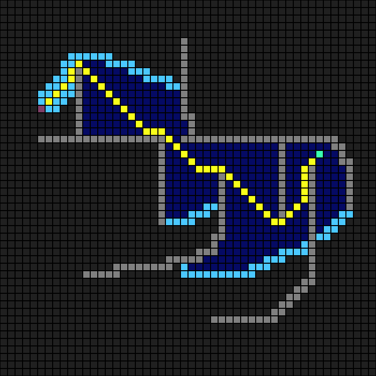 The figure shows a path computed with A* with its typical area of explored squares around the optimal path.
This grid is an example of a uniform cost grid. Traveling a rectangle horizontally or vertically has a distance of 1, traveling diagonally to a neighbour has length sqrt(2). (The code uses 10/2 and 14/2 as relative approximation.) The distance between two neighbouring nodes in the same direction is the same everywhere. A* performs quite badly with uniform cost grids.
Every node has eight neighbours. All those neighbours are tested against the open and closed lists. The algorithm behaves as if each node is in a completely separate world, expanding in all directions, and storing every node in the open or closed list. In other words, every explored rectangle in the picture above has been added to the closed list.
Many of them also have been added to the open list at some point in time. While A* 'walks' towards the end node, the traveled path gets longer and the estimated path gets shorter. There are however in general a lot of feasible parallel paths, and every combination is examined and stored.
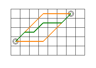
In the figure, the shortest path between the left starting point and the right destination point is any sequence of right-up diagonal or right steps, within the area of the two yellow lines, for example the green path. As a result, A* spends most of its time in handling updates to the open and closed lists, and is very slow on big open fields where all paths are equal.
Jump point search algorithm
The JPS algorithm improves on the A* algorithm by exploiting the regularity of the grid. You don't need to search every possible path, since all paths are known to have equal costs. Similarly, most nodes in the grid are not interesting enough to store in an open or closed list. As a result, the algorithm spends much less time on updating the open and closed lists. It potentially searches larger areas, but the authors claim the overall gain is still much better better due to spending less time updating the open and closed lists.
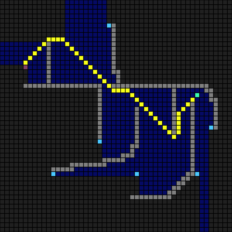
This is the same search as before with the A* algorithm. As you can see you get horizontal and vertical searched areas, which extend to the next obstacle. The light-blue points are a bit misleading though, as JPS often stacks several of them at the same location.
The algorithm
The JPS algorithm builds on the A* algorithm, which means you still have an estimate function, and open and closed lists. You also get the same optimality properties of the result under the same conditions. It differs in the data in the open and closed lists, and how a node gets expanded. The paper discussed here finds paths in 2D grids with grid cells that are either passable or non-passable. Since this is a common and easy to explain setup, this article limits itself to that as well. The authors have published other work since 2011 with extensions which may be interesting to study if your problem is different from the setup used here.
Having a regular grid means you don't need to track precise costs every step of the way. It is easy enough to compute it when needed afterwards. Also, by exploiting the regularity, there is no need to expand in every direction from every cell, and have expensive lookups and updates in the open and closed lists with every cell like A* does. It is sufficient to only scan the cells to check if there is anything 'interesting' nearby (a so-called jump point). Below, a more detailed explanation is given of the scanning process, starting with the horizontal and vertical scan. The diagonal scan is built on top of the former scans.
Horizontal and vertical scan
Horizontal (and vertical) scanning is the simplest to explain. The discussion below only covers horizontal scanning from left to right, but the other three directions are easy to derive by changing scanning direction, and/or substituting left/right for up/down.
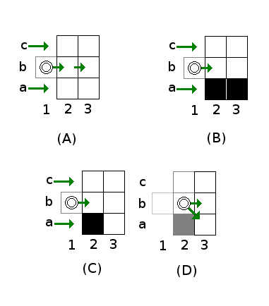
The (A) picture shows the global idea. The algorithms scans a single row from left to right. Each horizontal scan handles a different row. In the section about diagonal scan below, it will be explained how all rows are searched.
At this time, assume the goal is to only scan the b row, rows a and c are done at some other time. The scan starts from a position that has already been done, in this case b1. Such a position is called a parent. The scan goes to the right, as indicated by the green arrow leaving from the b1 position. The (position, direction) pair is also the element stored in open and closed lists. It is possible to have several pairs at the same position but with a different direction in a list.
The goal of each step in the scan is to decide whether the next point (b2 in the picture) is interesting enough to create a new entry in the open list. If it is not, you continue scanning (from b2 to b3, and further). If a position is interesting enough, new entries (new jump points) are made in the list, and the current scan ends.
Positions above and below the parent (a1 and c1) are covered already due to having a parent at the b1 position, these can be ignored. In the [A] picture, position b2 is in open space, the a and c rows are handled by other scans, nothing to see here, we can move on [to b3 and further]. The picture is the same.
The a row is non-passable, the scan at the a row has stopped before, but that is not relevant while scanning the b row.
The [C] picture shows an 'interesting' situation. The scan at the a row has stopped already due to the presence of the non-passable cell at a2 [or earlier]. If we just continue moving to the right without doing anything, position a3 would not be searched. Therefore, the right action here is to stop at position b2, and add two new pairs to the open list, namely (b2, right) and (b2, right-down) as shown in picture [D]. The former makes sure the horizontal scan is continued if useful, the latter starts a search at the a3 position (diagonally down).
After adding both new points, this scan is over and a new point and direction is selected from the open list. The row below is not the only row to check. The row above is treated similarly, except 'down' becomes 'up'.
Two new points are created when c2 is non-passable and c3 is passable. (This may happen at the same time as a2 being non-passable and a3 being passable. In that case, three jump points will be created at b2, for directions right-up, right, and right-down.)
Last but not least, the horizontal scan is terminated when the scan runs into a non-passable cell, or reaches the end of the map. In both cases, nothing special is done, besides terminating the horizontal scan at the row.
Code of the horizontal scan
def search_hor(self, pos, hor_dir, dist):
  """ Search in horizontal direction, return the newly added open nodes
  @param pos: Start position of the horizontal scan.
  @param hor_dir: Horizontal direction (+1 or -1).
  @param dist: Distance traveled so far.
  @return: New jump point nodes (which need a parent). """

  x0, y0 = pos

  while True:
    x1 = x0 + hor_dir
    if not self.on_map(x1, y0):
      return []

    # Off-map, done.
    g = grid[x1][y0]
    if g == OBSTACLE: return []

    # Done.
    if (x1, y0) == self.dest:
      return [self.add_node(x1, y0, None, dist + HORVERT_COST)]

    # Open space at (x1, y0).
    dist = dist + HORVERT_COST
    x2 = x1 + hor_dir
    nodes = []

    if self.obstacle(x1, y0 - 1) and not self.obstacle(x2, y0 - 1):
      nodes.append(self.add_node(x1, y0, (hor_dir, -1), dist))

    if self.obstacle(x1, y0 + 1) and not self.obstacle(x2, y0 + 1):
      nodes.append(self.add_node(x1, y0, (hor_dir, 1), dist))

    if len(nodes) > 0:
      nodes.append(self.add_node(x1, y0, (hor_dir, 0), dist))

    return nodes # Process next tile. x0 = x1
oordinate (x0, y0) is at the parent position, x1 is next to the parent, and x2 is two tiles from the parent in the scan direction. The code is quite straightforward.
After checking for the off-map and obstacle cases at x1, the non-passable and passable checks are done, first above the y0 row, then below it. If either case adds a node to the nodes result, the continuing horizontal scan is also added, all nodes are returned. The code of the vertical scan works similarly.
Diagonal scan
The diagonal scan uses the horizontal and vertical scan as building blocks, otherwise, the basic idea is the same. Scan the area in the given direction from an already covered starting point, until the entire area is done or until new jump points are found.
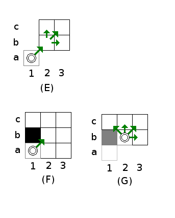
The scan direction explained here is diagonally to the right and up. Other scan directions are easily derived by changing 'right' with 'left', and/or 'up' with 'down'. Picture [E] shows the general idea.
Starting from position a1, the goal is to decide if position b2 is a jump point. There are two ways how that can happen. The first way is if a2 (or b1) itself is an 'interesting' position. The second way is if up or to the right new jump points are found.
The first way is shown in picture [F]. When position b1 is non-passable, and c1 is passable, a new diagonal search from position b2 up and to the left must be started. In addition, all scans that would be otherwise performed in the diagonal scan from position a1 must be added. This leads to four new jump points, as shown in picture [G].
Note that due to symmetry, similar reasoning causes new jump points for searching to the right and down, if a2 is non-passable and a3 is passable. (As with the horizontal scan, both c1 and a3 can be new directions to search at the same time as well.) The second way of getting a jump point at position b2 is if there are interesting points further up or to the right.
To find these, a horizontal scan to the right is performed starting from b2, followed by a vertical scan up from the same position. If both scans do not result in new jump points, position b2 is considered done, and the diagonal scan moves to examining the next cell at c3 and so on, until a non-passable cell or the end of the map.
Code of the diagonal scan
def search_diagonal(self, pos, hor_dir, vert_dir, dist):
  """ Search diagonally, spawning horizontal and vertical searches. Returns newly added open nodes.
  @param pos: Start position.
  @param hor_dir: Horizontal search direction (+1 or -1).
  @param vert_dir: Vertical search direction (+1 or -1).
  @param dist: Distance traveled so far.
  @return: Jump points created during this scan (which need to get a parent jump point). """
  x0, y0 = pos
  while True:
    x1, y1 = x0 + hor_dir, y0 + vert_dir

    if not self.on_map(x1, y1):
      return []

    # Off-map, done.
    g = grid[x1][y1]
    if g == OBSTACLE:
      return []

    if (x1, y1) == self.dest:
      return [self.add_node(x1, y1, None, dist + DIAGONAL_COST)]

    # Open space at (x1, y1)
    dist = dist + DIAGONAL_COST x2, y2 = x1 + hor_dir, y1 + vert_dir
    nodes = []

    if self.obstacle(x0, y1) and not self.obstacle(x0, y2):
      nodes.append(self.add_node(x1, y1, (-hor_dir, vert_dir), dist))

    if self.obstacle(x1, y0) and not self.obstacle(x2, y0):
      nodes.append(self.add_node(x1, y1, (hor_dir, -vert_dir), dist))
      hor_done, vert_done = False, False

    if len(nodes) == 0:
      sub_nodes = self.search_hor((x1, y1), hor_dir, dist)
      hor_done = True

    if len(sub_nodes) > 0:
      # Horizontal search ended with a jump point.
      pd = self.get_closed_node(x1, y1, (hor_dir, 0), dist)

      for sub in sub_nodes:
        sub.set_parent(pd)

      nodes.append(pd)

      if len(nodes) == 0:
        sub_nodes = self.search_vert((x1, y1), vert_dir, dist)
        vert_done = True

        if len(sub_nodes) > 0:
          # Vertical search ended with a jump point.
          pd = self.get_closed_node(x1, y1, (0, vert_dir), dist)
          for sub in sub_nodes:
            sub.set_parent(pd)
            nodes.append(pd)

          if len(nodes) > 0:
            if not hor_done:
              nodes.append(self.add_node(x1, y1, (hor_dir, 0), dist))

              if not vert_done:
                nodes.append(self.add_node(x1, y1, (0, vert_dir), dist))

                nodes.append(self.add_node(x1, y1, (hor_dir, vert_dir), dist))

              	return nodes # Tile done, move to next tile. x0, y0 = x1, y1
The same coordinate system as with the horizontal scan is used here as well. (x0, y0) is the parent position, (x1, y1) is one diagonal step further, and (x2, y2) is two diagonal steps. After map boundaries, obstacle, and destination-reached checking, first checks are done if (x1, y1) itself should be a jump point due to obstacles. Then it performs a horizontal scan, followed by a vertical scan. Most of the code is detection that a new point was created, skipping the remaining actions, and then creating new jump points for the skipped actions. Also, if jump points got added in the horizontal or vertical search, their parent reference is set to the intermediate point. This is discussed further in the next section.
Creating jump points
Creating jump points at an intermediate position, such as at b2 when the horizontal or vertical scan results in new points has a second use. It's a record of how you get back to the starting point. Consider the following situation
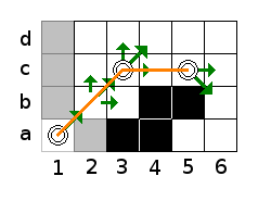
Here, a diagonal scan started at a1. At b2 nothing was found. At c3, the horizontal scan resulted in new jump points at position c5. By adding a jump point at position c3 as well, it is easy to store the path back from position c5, as you can see with the yellow line. The simplest way is to store a pointer to the previous (parent) jump point. In the code, I use special jump points for this, which are only stored in the closed list (if no suitable node could be found instead) by means of the get_closed_node method.
Starting point
Finally, a small note about the starting point. In all the discussion before, the parent was at a position which was already done. In addition, scan directions make assumptions about other scans covering the other parts. To handle all these requirements, you first need to check the starting point is not the destination. Secondly, make eight new jump points, all starting from the starting position but in a different direction. Finally pick the first point from the open list to kick off the search.
Performance
I haven't done real performance tests. There is however an elaborate discussion about it in the original paper. However, the test program prints some statistics about the lists.
Dijkstra: open queue = 147
Dijkstra: all_length = 449
A*: open queue = 91
A*: all_length = 129
JPS: open queue = 18
JPS: all_length = 55
The open/closed list implementation is a little different. Rather than moving an entry from the open to the closed list when picking it from the open list, it gets added to an overall list immediately. This list also knows the best found distance for each point, which is used in the decision whether a new point should also be added to the open list as well. The all_length list is thus open + closed together.
To get the length of the closed list, subtract the length of the open list. For the JPS search, a path back to the originating node is stored in the all_length list as well (by means of the get_closed_node). This costs 7 nodes.
As you can see, the Dijkstra algorithm uses a lot of nodes in the lists. Keep in mind however that it determines the distance from the starting point to each node it vists. It thus generates a lot more information than either A* or JPS. Comparing A* and JPS, even in the twisty small area of the example search, JPS uses less than half as many nodes in total. This difference increases if the open space gets bigger, as A* adds a node for each explored point while JPS only add new nodes if it finds new areas behind a corner.
References
The Python3 code is attached to the article. Its aim is to show all the missing pieces of support code from the examples I gave here. It does not produce nifty looking pictures. Dijkstra algorithm Not discussed but a worthy read.
- (Article at Gamedev)
A* algorithm
- http://theory.stanford.edu/~amitp/GameProgramming/AStarComparison.html
- (Article at Gamedev)
JPS algorithm
- (Wikipedia on JPS) http://en.wikipedia.org/wiki/Jump_point_search
- (Published article) harabor-grastien-aaai11.pdf
Versions
- 20151024 First release


Thanks for the write-up; it's a neat algorithm. I'd like to share some javascript JPS tests I put together a few years ago. These have crude graphics and some timing/debug output in the browser console.
http://tnovelli.net/junk/mwtests/jps1.html
http://tnovelli.net/junk/mwtests/jps2.html
It's definitely faster than vanilla A*. I don't have a test for that, but I remember it being "seconds" in javascript. JPS test #1 is typically 1-10ms, approaching 1 second in the worst case (northeast hall to just outside the southwest wall). Test #2 has some tweaks to bail out early.
This works fine for player movement in an RPG. Could work well for combat AI too; it has a nice tendency to zigzag and hide behind corners.
For general AI it would need to find a path to any reachable point. For example it can't get from one side of a wall/obstacle to the other. That may be an "optimization" in my scanning function, not a limitation inherent in JPS.