Overview

Navigation graph remains a useful alternative to navigation mesh and may offer certain advantages depending on a game's environment. This article discusses several approaches to navigation graph generation: from an automated one based on Delaunay triangulation to a completely automatic method derived from triangulation of navigable areas and dual graph of triangulation.

The article uses general computational geometry algorithms and also algorithms inspired by image processing. An open source computer vision library OpenCV ([Bradski2008], [OCV]) may be used to implement image processing-based techniques discussed here.

We also touch on hierarchical navigation graphs that open important optimization opportunities.

Introduction: Navigation Meshes and Graphs

There is a growing number of middle-ware products handling navigation of game agents. We are not going to review or even attempt to mention any of them. While they may provide solid solutions for many typical situations, building a custom navigation system may be still the only viable option for many projects. Hence it is important to understand what techniques engineers and designers can choose from.

There are two main approaches to creating and supplying navigation (aka "routing", or "pathfinding") information for game levels. One is based on navigation meshes and the other is using the navigation graph (see general overview of the methods to represent navigation data in [Stout2000] and also [Snook2000] for navigation meshes in particular). Figure 1 below shows examples of both kinds of navigation data representing a navigable area for the same test environment.

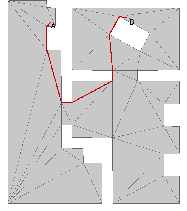
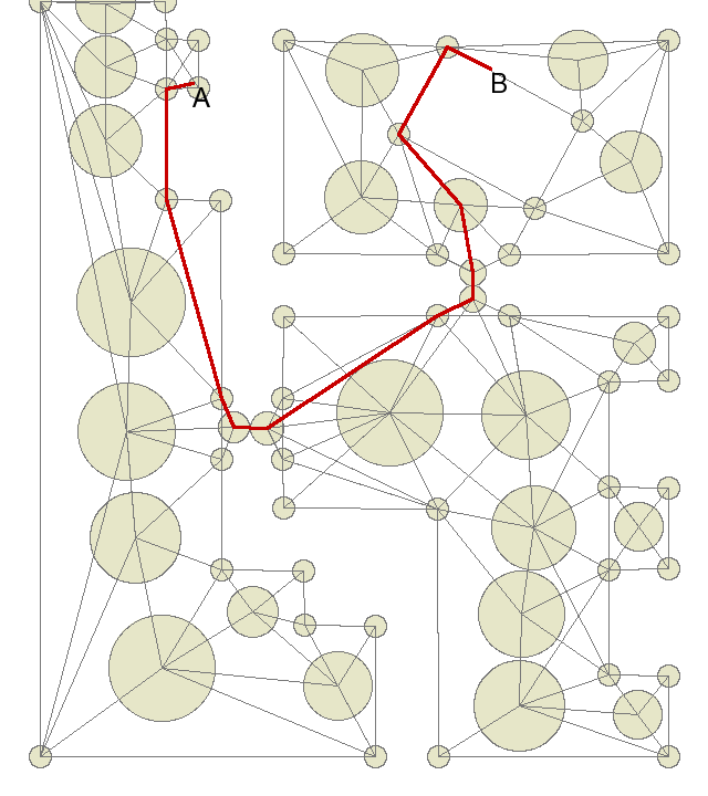
Figure 1. Navigation Mesh and Navigation Graph with a path connecting points A and B.

Navigation Mesh

Agents in game can use a navigation mesh to find the path from location A to location B by an algorithm which we outline in very general terms. First, given the initial agent's location A, the algorithm finds what triangle Ta of the mesh contains A and what triangle Tb contains B (the destination). Then, a shortest path across the mesh can be built. This path is a list L of connected triangles from triangle Ta to triangle Tb. Usually this is done using A* (a-star) algorithm (see [Matthews2002] for an excellent introduction into A*).

Since any paths inside navigation triangles are valid, knowing the list L allows us to connect A to B with a piece-wise linear path. Hence, the calculation of L accomplishes our task, at least in its first rough approximation. Usually further manipulations of the path are desirable as this rough path looks too robotic. This issue is quite obvious from the figure above. While improving aesthetics of the path is a fascinating topic, we will not go any deeper on this.

Navigation meshes can often be naturally derived from collision geometry in an automated or completely automatic manner. It can be updated in run time as well, but this may be challenging due to the performance constraints unless we deal with only small portions of the mesh at a time.

Navigation Graph

Navigation graph approaches the problem of building navigation data from a dual perspective. Yet the techniques involved are often similar in many ways to a mesh-based approach.
Namely, the graph is based on nodes, which are not intended to cover all navigable geometry but rather provide useful markers and serve as waypoints. A set of 2D primitives (circles, quads and the like) can be used to represent nodes in a navigation graph. Any path inside a node is considered valid. Also, a path (usually - a straight line) from any point in the environment to any point inside any node is considered to be valid provided it satisfies some additional constraints. The most common constraint is that the path does not intersect collision geometry. Additionally, we may exclude high drops, too steep slopes, water surfaces, etc.

More often than not, checking against collision and other terrain properties along the path could be expensive. Such checks can be replaced by checking against much simpler representations of un-navigable geometry via blocking primitives. The blocking primitives are by far less-detailed and are often limited to boxes (oriented or axis-aligned) and cylinders. This allows for very efficient testing of ray intersection against blocking primitives. Note that the navigation mesh usually doesn't require addition of blocking primitives as all information about the navigable area is already included in the navigation mesh.

Below, Figure 2 shows an example of blocking primitives which are semi transparent red axis-aligned boxes with white outlines placed along the walls, trash cans and other obstacles. The navigation graph has yellow-green nodes connected with bright yellow edges. The area shown approximately corresponds to the lower left corner of the test environment on Figure 1. (The door is not unlocked yet so there is no connection to the indoors part of the test environment.)

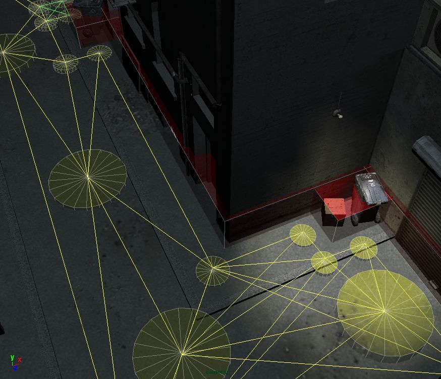
Figure 2 Blocking Primitives and Navigation Graph (Environment model: courtesy of Inna Cherneykina.)

Given a navigation graph and a set of blocking primitives, we can construct a path using the following algorithm: From starting point A we look for the closest navigation node Na such that the line of view from A to Na is not blocked by any primitive. In a similar manner we find node Nb for destination point B. Then using a-star we find a list of nodes connecting Na to Nb. On the figure below the navigation graph from Figure 1 is shown together with blocking primitives (pale pink boxes).

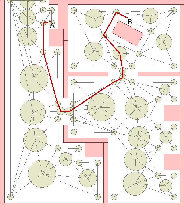
Figure 3 Navigation Graph and Blocking Primitives

Navigation graphs may offer certain advantages over navigation meshes. To start with, the graph can easily incorporate navigation slots of objects placed into the environment. Say, we need an agent to approach a door and orient itself in a certain way to successfully open it. With navigation graphs the slots indicating desired position near the door can become just another node in the graph, likely with some additional attributes (orientation, and may also contain an indication of what type of animation to use for opening the door, etc.)

Second, since the navigation graph is not tied to the level geometry in the same direct way as navigation mesh, it can offer extra flexibility during level design. The nodes are usually represented as objects in the level design tools. As such they can be easier manipulated than triangles in a navigation mesh where designers should care about preserving topological properties of the mesh. By tweaking graph nodes location the designer can introduce certain subtle (and not so subtle) desirable effects influencing pathing in the environment.

Needless to say, manual generation of a navigation graph and its tweaking can be very time consuming. Another downside is that such handcrafted graphs are difficult to update if the geometry changes during the design process and they require extra care in case of run-time modifications in game.

Summarizing, we may conclude that a navigation mesh is more appropriate when navigation data is generated automatically and a navigation graph may be more preferred when level designers' input is needed or necessary. This leads to the necessity of simplifying creation and maintenance of the navigation graph when it is subject to manual modification.

Manual creation of navigation graph and its validation

There are several technical considerations to take into account while creating a navigation graph.

Optimal density of the graph

On one hand the graph has to be dense enough in the environment to provide navigable nodes accessible from each valid location. On the other hand an excessively-detailed graph is hard to build manually and may lead to longer a-star calculation times. Also it tends to result in a robotic look of agents: they tend to stick to nodes without taking obvious shortcuts.

Surprisingly a sparse graph may also lead to an increase of run-time calculations or even breaking down of the algorithm if it does not take into consideration the following situation - see Figure 4.

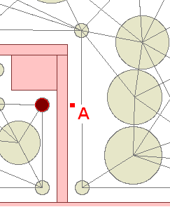
Figure 4 Picking nearest node on the other side of the wall

On Figure 4 the agent is placed at location A. When looking for the nearest node it would pick the one highlighted in red. Obviously it is the wrong node to start a path with. Hence a sanity check for intersection of the ray agent-selected node against blocking primitives would be needed to prevent the agent running into the wall on its way to the highlighted node. But then, if the selected node is rejected, we need to find another one which is nearby yet reachable directly. There may be an expensive calculation involved in this additional search, depending on the complexity of the environment.

Hence an off-line procedure validating the navigation graph may also check for such gaps in the graph rather than rely on run-time code to recover from lack of nodes.

Taking into account finite size of the agents

Next, edges of the navigation graph have to be placed in such a way that following along them would keep agents sufficiently far from any collision geometry. Generally, as soon as an agent reaches node N[sub]i[/sub] on its path, it can immediately turn towards the next node N[sub]i+1[/sub], see Figure 5. On this figure collision with geometry outlined by a blocking primitive may occur along the highlighted path from A to B. On the left side of this Figure some paths between N[sub]i[/sub] and N[sub]i+1[/sub] are ok but many are blocked as shown.

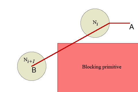
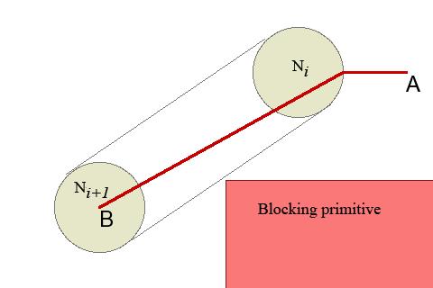
Figure 5 Transition between nodes:
(left) the agent may turn at distance R from the node center;
(right) a wider corridor has to be clear of obstacles.

Thus, it's not only the edges of the graph but a wider area between each of the two connected nodes has to be clear of obstacles. This area is a 2D cylinder with the bases at the nodes and sides defined by external mutual tangents. It is not always easy to satisfy this requirement when creating a navigation graph manually.

A useful technique to keep agents from coming too close to the walls is a method based on Minkowski sums and is widely adopted in robotics [deBerg2010]. The main idea behind this approach can be explained in simplified terms as follows: Suppose that an agent has a bounding sphere of radius R, which we will also call the agent's radius. Apparently we want to keep an agent away from walls at a distance of at least R. Also suppose that originally blocking primitives were created exactly aligned with the collision geometry. If we "inflate" the primitives by adding R on each side along each dimension, and shrink the navigable area correspondingly by the same amount, we may represent the agent as a point. Conveniently this will keep the agent away from the actual collision geometry during navigation. The procedure of inflating blocking primitives and shrinking navigable areas can be done automatically in the development pipeline (preferably) or in run-time. The figure below illustrates this technique. Lighter-color blocking primitives were obtained from original ones using such inflation.

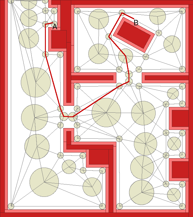
Figure 6 Inflated Blocking Primitives (light red) overlaid with original
primitives (dark red) and navigation graph

To summarize this section, it is better to avoid completely manual creation of navigation graphs as it is an error-prone and time-consuming process. As an alternative we should look for completely automatic techniques or, sometimes, the combination of manual steps with automated procedures. From this perspective it was worth outlining manual steps of navigational graph creation to flesh out the main constraints.

Connecting nodes via triangulation algorithms

Out of all manual steps, placing nodes without actually connecting them by edges is the easier and faster part of the task. Luckily it is possible to automate connecting existing nodes in an environment that already contains blocking primitives. Delaunay triangulation [deBerg2010] provides one of the possible solutions.

Triangulation of a planar set of points connects them by edges in such a way that no edges intersect each other (planarity of connection graph) and no more edges can be added without breaking this condition (maximal property). Delaunay triangulation offers some additional benefits: it maximizes minimal angle of all the triangles in the triangulation. Thus it tends to produce least amount of "thin" triangles. This property by itself may not seem to be very important but it comes from the fact that Delaunay triangulation is a dual object for Voronoi diagram [deBerg2010].

A Voronoi diagram of a discrete set of N points (nodes) on a plane can be defined as subdivision of the plane into N regions (aka Dirichlet domains) by finding the nearest node for each point on a plane. If a point is on equal distance d from two or more nodes N[sub]i1[/sub],...,N[sub]ik[/sub], and no other nodes are closer than d then it belongs to the boundary of the corresponding domains.

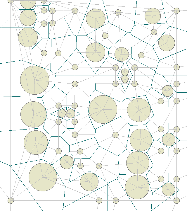
Figure 7 Voronoi cells and Delaunay Triangulation (no blocked edges
removed) for the graph nodes

Voronoi diagrams appear naturally in tasks like optimal placement of retail stores in a neighborhood to minimize travel distance to them, or placing re-translators for wireless networks. Pretty much any modern book on computational geometry has at least a chapter or two on both Delaunay triangulation and Voronoi diagrams so we will not spend more time on the definitions or examples.

A Voronoi diagram of the navigation nodes shows which node will be picked for each starting point when searching for the first node on the path hence its obvious importance for building navigation graphs and placing nodes. As a side note, consider Voronoi cells overlaid over blocking primitives in the problematic area from Figure 4

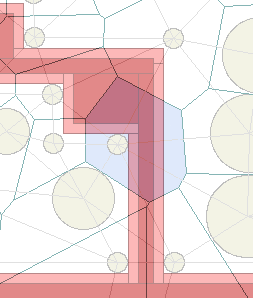
Figure 8 Voronoi cells overlaid over blocking primitives.
Blue shaded cell extends beyond blocking primitive and creates problematic
situation shown on Figure 4.

Such overlay of Voronoi cells over blocking primitives can easily reveal too sparse placement of the nodes with respect to the blocking primitives. A formal requirement for correct placement of nodes with respect to the primitives to ensure that all nearest nodes are immediately reachable is the following: If V is Voronoi cell corresponding to a node N, and Bi are blocking primitives, i=1,..,M, and \ is set-theoretical subtraction then we need a set V' = V \ (union of all Bi) obtained by subtracting from V all of the blocking primitives to be convex and the node N must belong to it.

There are a number of algorithms for building Delaunay triangulation and corresponding Voronoi subdivisions. For practical purposes we can use available implementations like the one coming with the OpenCV library [Bradski2008], [OCV]. Alternatively we can adopt implementations described in text books like [ORourke2000]. While sub-optimal in terms of complexity, these implementations provide sufficient performance for most practical purposes when the number of nodes is not too high. Using hierarchical graphs when possible will make Delaunay triangulation task tractable even for quite big environments.

After Delaunay triangulation is built, the edges of the graph intersecting blocking primitives are removed. Removal of edges intersecting blocking primitives may uncover nodes placed problematically from the point of view of finding the nearest initial node in the graph. Connection between nodes C and D is conspicuously missing from the graph suggesting that Voronoi cells for these nodes may not have enough coverage to include all points like A on Figure 4. There are few more similarly missing edges of the graph and sure enough all of them indicate problems with nodes layout.

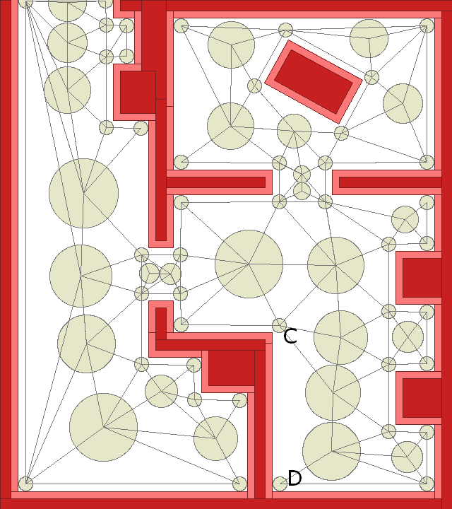
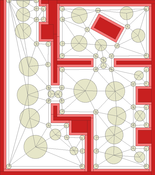
Figure 9 Navigation graphs obtained from Delaunay triangulation by
removing edges blocked by primitives. "Missing" edges on the left (like
between nodes C and D) indicate problematic placement of nodes fixed on
the right version of the graph.

It is worth mentioning that hierarchical approach to graph construction and to the search of the nearest node alleviates the problem of picking the wrong initial node based on proximity alone. We will elaborate on this it in the section on hierarchical navigation graphs.

Sometimes it is necessary to include particular edges into the final triangulation. This variation of the Delaunay triangulation problem is called constrained and is considerably more difficult [Seidel1988]. However, for navigation purposes, we may have enough freedom to just add new edges after the initial navigation graph is built.

Navigable areas from collision geometry

It is useful to extract navigable areas from collision geometry as a polygonal mesh regardless of what is the target representation: navigation graph or navigation mesh. Navigation mesh can be directly created from this data but the navigation graph would require several additional steps that we will discuss later.

To create such polygonal representation we may consider rendering collision geometry into a sufficiently high resolution bitmap. It can be achieved by running rendering in the modeling application used as a level design tool or procedurally, directly from the scene data.

In most of the simpler cases the level geometry can be projected onto a plane without overlaps (e.g. a single floor of a building, or an outdoor terrain without caves or overhangs). The entire horizontal collision geometry can be rendered onto a horizontal plane using orthographic projection in one color (say, blue) and the vertical collision elements (walls and obstacles) can be rasterized as 1-pixel wide lines of different color (say, red), so that we can tell obstacles from navigable parts.

Since there are so many variations on the tools and modeling applications used in game development, we will skip discussion of the rendering step. We will assume that we already have a reasonably detailed map of flat pieces of collision geometry. It is also necessary to obtain a coordinate transformation allowing conversion of pixel coordinates into in-game coordinates (say, (x,y) scene coordinates).

Next after rendering, a flood fill algorithm in 2D raster image can be applied. Different variations of flood fill algorithms may work for this purpose. In OpenCV a result similar to flood fill may be achieved via (adaptive) threshold operation. (Look up cvThershold and cvAdaptiveThreshold: the first one will almost surely cover all your needs). We don't go into details because of highly diverse source of the bitmaps due to the diversity of modeling tools and methods but the idea behind converting the rendered image into binary image of navigable areas is mostly self-evident and technically not too difficult.

As an aside note, we may use the rendered source image to inflate one-pixel width blocking lines by half width of the max dimension of the agent radius. This can be done using OpenCV dilate operation. On the other hand, we can delay this until later steps when we obtain polygonal representation of the navigable area.

Polygonization of a binary image can be handled via contour detection. Here we outline the algorithm using Python (OpenCV now conveniently ships with pre-built Python binding).

1. Create binary image of the navigable area (namely, 8bit single channel black and white image) by rendering environment with appropriate settings. We start below with ready image on Figure 10.
   [nbsp]
   
2. Run contours extraction. This requires steps:
   [bquote][font=Courier New][color=#000080]image = cv.LoadImage(navigableArea)
   storage = cv.CreateMemStorage(0)
   contours = cv.FindContours(image, storage,
   [nbsp][nbsp][nbsp][nbsp][nbsp][nbsp][nbsp][nbsp][nbsp][nbsp][nbsp][nbsp][nbsp]cv.CV_RETR_CCOMP, cv.CV_CHAIN_APPROX_SIMPLE)
   contours = cv.ApproxPoly(contours, storage, cv.CV_POLY_APPROX_DP, 3, 1)[/color][/font][/bquote]
   

A call to ApproxPoly simplifies found contours by converting them to polygons, which is exactly our goal. After this call we will have polygonal contours as list of vertices as (x,y) pairs of the first top level contour.

Accessing siblings and nested contours via contours.v_next() and contours.h_next() would allow us to iterate through all the found contours. Another useful function is DrawContours. It provides an easy visualization of contours. Below on the Figure 10 we used custom visualization to show vertices.

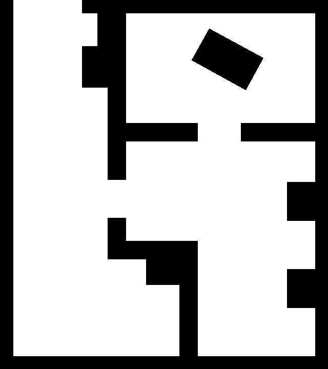
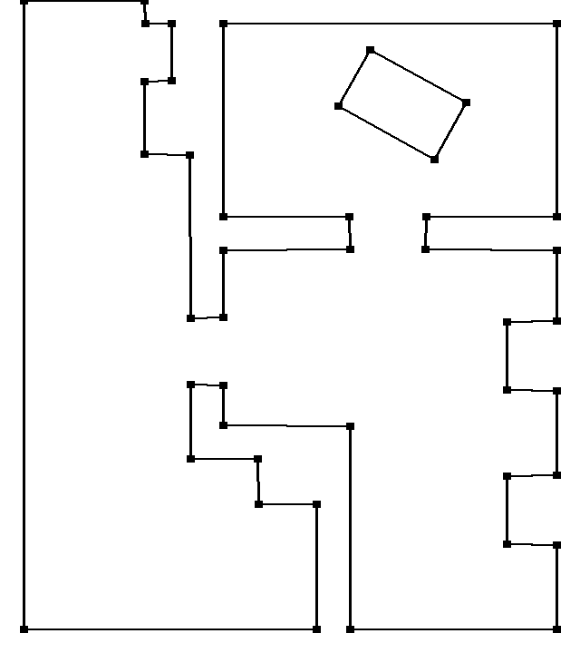
Figure 10 Extracting contours from binary image. The contours hierarchy
has single contour on the top level and total depth =1 because of single
inner contour (rotated rectangle).

We have several options on how to proceed next with building polygonal mesh from the contours. Ideally we want to obtain triangular mesh, and this is a well known problem of polygon triangulation [dBerg2010], [Orourke2000]. Our situation is a bit more complex as our polygons may have holes. Also one of our objectives is to have triangulation similar to Delaunay triangulation (no excessively skinny triangles). Yet using constrained Delaunay triangulation may be an algorithmic overkill. Though not optimal in terms of performance (complexity is at least that one of Delaunay triangulation), we may consider the following step:

• Run Delaunay triangulation on the vertices of extracted contours. Tessellate Delaunay mesh using contours to include edges and corresponding triangles from the extracted contours (Figure 11).
  

Tessellation must ensure that the resulting mesh is flat and triangular. The easiest way to achieve this is to intersect all contour edges with Delaunay tessellation vertices to check if there are non-trivial intersections indicating that the current mesh is not flat.

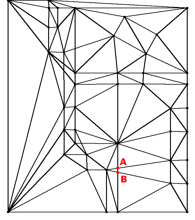
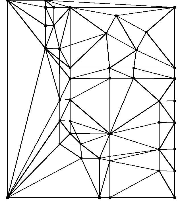
Figure 11 Delaunay mesh with added contours on the left is not flat: points
A and B mark intersecting edges. Adding vertices at the locations A and B
and repeating triangulation flattens the mesh (right).

Finally, we complete procedure with the step:

• Eliminate edges and faces that are not covering navigable terrain (Figure 11 right). The result is shown on the Figure below.
  

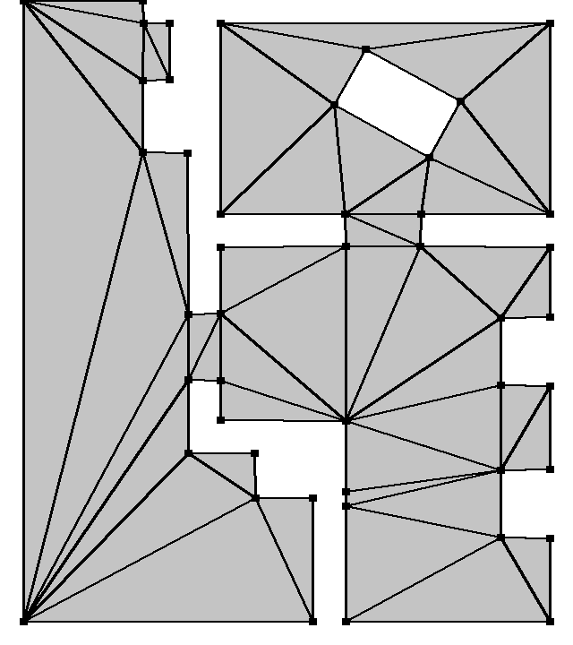
Figure 12 Triangulation of navigable area. This mesh may be optionally
optimized or tessellated further.

Concluding our discussion of extraction of the navigable area as a polygonal mesh, we should mention that OpenCV algorithms work particularly well with computer generated images such as those obtained from level design tools. This makes them a robust element of the game pipeline.

As a side note, to compare this "sterile" setup with real world applications of OpenCV check out an article [Botana2010]. It provides an excellent coverage of contours detection and their handling. It is related to real-world images for augmented reality games. Working with images acquired with a camera is much more challenging.

Automatic placement of nodes for navigable areas

So far we completed triangulation of navigable area. Such triangular mesh can be easily converted into navigation mesh by augmenting it with explicit connectivity information if necessary. We could be done at this point if we decide to go with navigation mesh, but we can also use triangulation for building a navigation graph.

"Art gallery" navigation graph

Given some triangulation of the navigable area we can follow a minimalist approach and use the results of the art gallery theorem [deBerg2010], [ORourke200]. It asks for placing minimal number of guards in a polygonal shaped gallery so that all of the walls are seen by a guard. The additional twist here is that we may have holes in our polygonal representation so generally we are not dealing with simple polygons as in the basic art gallery theorem.

The requirement of visibility posed by the art gallery theorem is exactly the one we want to satisfy for nodes on the first step of path finding (find nearest visible). If the nodes of the graph contain all of the guard locations then we have a graph which allows getting to a node from any navigable location. Note that the guards are not required to see each other so we may need to place additional nodes to complete the graph.

The main step in proving of the art gallery theorem is to triangulate the polygon. Triangulation from inflated blocking primitives was completed in the previous section so we will use it to place the nodes corresponding to the guards. The vertices of the triangulation are valid node positions by construction.

We can choose the first vertex arbitrarily or pick one of the highest order to cover maximum number of triangles. Next node can be placed by finding first triangle that is not entirely visible from any of the existing nodes.

Next we need to check for visibility of nodes from each other and use mesh connectivity to place intermediate nodes to ensure that the graph is correctly connected. Below is an example of such graph.

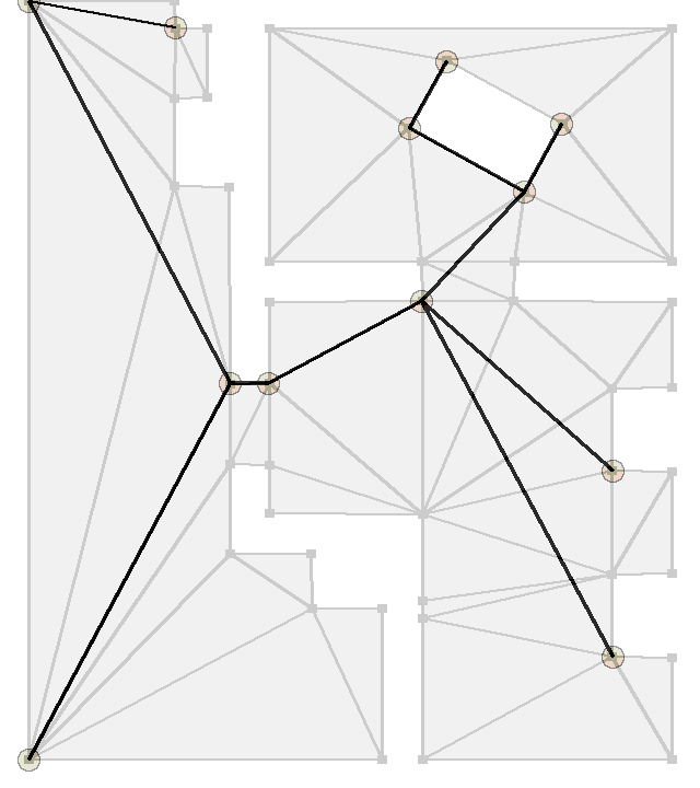
Figure 13 Graph based on Art Gallery Theorem

Despite being very small and yet valid representation of the navigable area, such a graph is not very useful as is. One of the main reasons is lots of backtracking that will occur during navigation with such graph i.e. agents would be often moving towards a node that is not in the intuitively correct direction of the goal. We discuss this issue in more details in the next section.

Dual graph approach

Dual graph of a triangular mesh [deBerg2010] can be another candidate for the navigation graph. It is built by associating a node with each triangle and then connecting nodes corresponding to the adjacent triangles. Geometrically, the nodes are usually placed at some internal point of the triangle, say, at its center of mass. Obviously, in such dual graph at least one of its nodes is "visible" from any point of the navigable area. However such graph may have problems as shown on the next Figure.

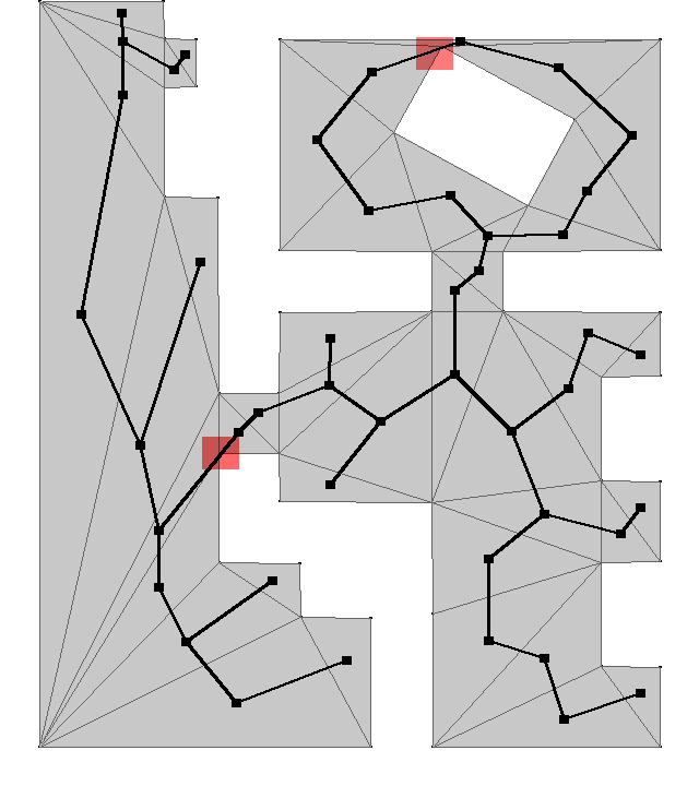
Figure 14 Dual graph of triangulation. Red highlights show possible
intersection of edges with blocking primitives.

The problem we encountered on the Figure above results from possible intersection of the edges of dual graph with blocking primitives. This can be relatively easy to detect and correct by connecting two triangles via an additional one of their common vertices. Also we can use inflated by the agent radius primitives to ensure that the edges of the dual graph are sufficiently far from the collision geometry.

Additionally we can also include vertices and edges of the triangulation into the navigation graph. The result of adding edges connecting dual graph vertices with triangulation vertices and edges of the triangulation is shown below.

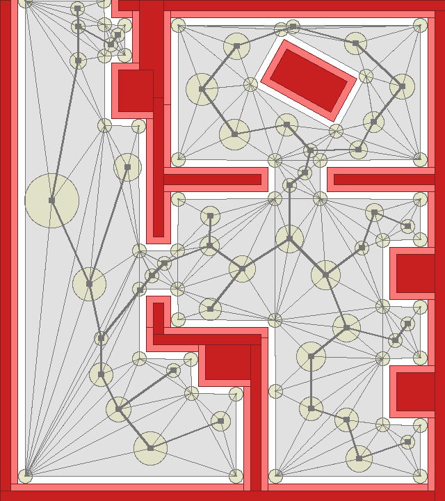
Figure 15 Extension of dual graph to corresponding navigation graph.

We can improve two aspects of the graph on Figure 15. Namely, both location and radius of nodes of dual graph can be picked more advantageously. Placing dual graph node at the incenter of the triangle (center of inscribed circle) and setting its radius to the radius of inscribed circle will give a better version of the graph (see Figure 16).

Note that overlapping nodes are not presenting a problem as any path inside a node radius is a valid path. Larger radius of the dual graph nodes would allow the agent to switch to the next node when following a path that includes dual graph node. Presence of the nodes corresponding to the vertices of the triangulated navigable area ensures that there will be no shortcuts across blocked areas due to too large dual nodes.

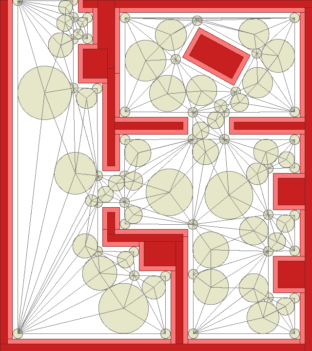
Figure 16 Placement of dual graph vertices at the incenter of triangle.
Radius of dual nodes set to the radius of the inscribed circle.

The graph shown on the Figure 16 may still present challenges in run-time: consider an agent starting path near the left-most bottom node of the graph and going into any other room. It would find the nearest node (left bottom node) and initially move towards it, and only after reaching it within the radius of the node the agent would turn to follow the path. This will present an obviously undesirable backtracking.

There are few approaches to this problem. One is to remove such redundant nodes (as obviously the graph will serve its purpose without corner nodes). But that will only make the problem slightly less obvious as there will be similar arrangements of nearest node and initial position leading to backtracking.

Another possible solution can be implemented in run time. After the path is calculated, we can check if the agent can start the path from Nth > 1 node by skipping the first few nodes. This will make pathfinding somewhat more expensive as we would need to run ray intersection tests against blocking primitives to ensure that shortcut is acceptable. On the other hand we would still need to do some path "beautification" to make it less robotic so this additional check may be not so expensive in comparison to other calculations we would need to perform.

In concluding this section we can tell that there are more ways to improve the graph on Figure 16, e.g. by reducing number of edges (redundant edges may result in slower run time performance of A*), better placement of nodes, etc. However the graph as we built it will perform reasonably well. Also it could be easily modified by level designers manually, if necessary, to meet their specific needs not covered by automatic graph generation.

Hierarchical graphs

Hierarchical navigation graphs come in handy when dealing with large environments with relatively loosely connected regions. In indoors environment, such connection is usually done via portals. Building "super-graph" with nodes corresponding to regions and edges to portals may greatly reduce load on A* when navigating between distant regions of the environment.

Indeed, first we can identify the super-node corresponding to the region where the agent is located and the super-node for the destination region. An A* run on super graph can return either "no path" if the regions are not connected, or a navigable path in super graph. This path consists of a list of regions the agent needs to visit in order to reach its destination. Navigation within each region is handled by a-star on regular graph.

Such optimization can be extremely helpful in particular in the cases when no path exists. Super-graph is much smaller and the absence of the path, if it happened to be the case, is learned at a much lower cost than exhaustive search on the regular navigation graph. This observation may seem not so important at the first glance but in practice most spikes in the navigation performance are usually coming from A* failing to find the path on a large graph.

Similar optimization is possible when we deal with open terrain and the regions are not so loosely connected. Still super graph would correctly reflect connectivity information on larger scale thus we can avoid expensive searches with negative outcome.

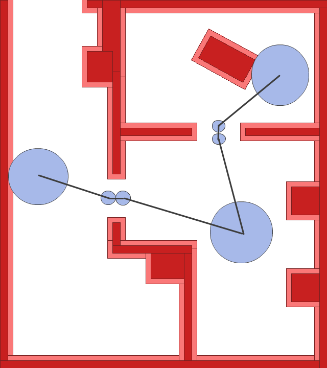
Figure 17 First super-level of navigation graph (left) of the graph on the
right.

Super nodes of the next level of the hierarchy of the navigation graph don't have to be placed at specific locations. But they are in logical correspondence to the regions they represent. The portal nodes (smaller blue nodes) also have to be in one-to-one correspondence of the portal nodes of the base navigation graph. Note that regions on the right are connected with single edge. This simplifies structure of the super-graph. Super graph still has to provide functionality to estimate distances to allow A* heuristics work efficiently.

Partitioning of the level into regions corresponding to the nodes of super graph has additional benefits. One of them is that we can worry less about situations like on Figure 4 when the nearest node is picked across blocked terrain. If the search for nearest node is limited to the current region then such situations will happen much less often and the search itself will speed up.

Apparently two-level hierarchy can be generalized to more levels but this is rarely justified in practice.

It is possible to come up with an automatic procedure to build a super graph from the original navigation graph but it is also often done manually. Hierarchical graphs are natural notion for graph-based navigation and reuse most of the code of the underlying a-star-based framework. Thus adding and supporting super graph can be quite easy and straightforward while performance advantages can be really dramatic. This may be a strong argument in favor of choosing graph-based approach for many types of environments.

Conclusion

In this article we focused on navigation graphs as a still-frequent solution to represent navigation data for games. The discussion covered several topics related to creation of navigation graphs for game environments based on different representation of navigable geometry in the game. Each stage of navigation graph creation contains a number of problems with deep roots in computational geometry. As we showed, insights from image processing can also benefit navigation graph creation.

While presented material is not sufficient to build a complete system, by far, it exposes some of the interesting aspects of the process and provides pointers to further research to those who are not relying on middle-ware for their routing needs.

Some of the approaches discussed here were applied to one of the projects the author worked in the past. Those approaches proved to be practical enough, not just of academic interest. Also the belief is that there are many more interesting topics in the area of navigation graph generation that can benefit game developers who are adventurous enough to go after custom solutions for their navigation needs.

References

[Botana2010] C?sar Botana "Electric Eye: Pattern Recognition in Augmented Reality", Game Developer Magazine, December 2010, pp.22-25

[Bradski2008] Garry Bradski, Adrian Kaehler "Learning OpenCV: Computer Vision with the OpenCV library" O'Reilly 2008, 555 pages

[deBerg2010] Mark de Berg et al, Computational Geometry: Algorithms and Applications, 3d edition, Springer, 2010, 386 pages.

[Matthews2002] James Matthews "Basic A* Pathfinding Made Simple" AI Game Programming Wisdom, Charles River Media 2002, pp. 105-103

[Snook2000] Greg Snook "Simplified 3D Movement and Pathfinding Using Navigation Meshes" in Game Programming Gems, Charles River Media, editor Mark DeLoura, 2000, pp. 288-304

[Stout2000] Bryan Stout "The Basics of A* for Path Planning" in Game Programming Gems, Charles River Media, editor Mark DeLoura, 2000, pp. 254-263

[OCV] OpenCV, an open source computer vision library available from SourceForge http://sourceforge.n...opencv-win/2.2/

[Orourke2000] J. O'Rourke "Computational Geometry in C" Cambridge University Press; 2000, 390 pages

[Seidel1988] R. Seidel. "Constrained Delaunay Triangulations and Voronoi Diagrams with Obstacles." Technical Report 260, Inst. for Information Processing, Graz, Austria, 1988