[size="5"] And There Was Light...

The funny thing about high technology is that sometimes it's hundreds of years old! For example, Calculus was independently invented by both Newton and Leibniz over 300 years ago. What used to be magic, is now well known. And of course we all know that geometry was invented by Euclid a couple thousand years ago. The point is that many times it takes years for something to come into "vogue". Neural Nets are a prime example. We all have heard about neural nets, and about what their promises are, but we don't really see too many real world applications such as we do for ActiveX or the Bubblesort. The reason for this is that the true nature of neural nets is extremely mathematical and understanding and proving the theorems that govern them takes Calculus, Probability Theory, and Combinatorial Analysis not to mention Physiology and Neurology.

The key to unlocking any technology is for a person or persons to create a Killer App for it. We all know how DOOM works by now, i.e. by using BSP trees. However, John Carmack didn't invent them, he read about them in a paper written in the 1960's. This paper described BSP technology. John took the next step an realized what BSP trees could be used for and DOOM was born. I suspect that Neural Nets may have the same revelation in the next few years. Computers are fast enough to simulate them, VLSI designers are building them right into the silicon, and there are hundreds of books that have been published about them. And since Neural Nets are more mathematical entities then anything else, they are not tied to any physical representation, we can create them with software or create actual physical models of them with silicon. The key is that neural nets are abstractions or models.

In many ways the computational limits of digital computers have been realized. Sure we will keep making them faster, smaller and cheaper, but digital computers will always process digital information since they are based on deterministic binary models of computation. Neural nets on the other hand are based on different models of computation. They are based on highly parallel, distributed, probabilistic models that don't necessarily model a solution to a problem as does a computer program, but model a network of cells that can find, ascertain, or correlate possible solutions to a problem in a more biological way by solving the problem a in little pieces and putting the result together. This article is a whirlwind tour of what neural nets are, and how they work in as much detail as can be covered in a few pages. I know that a few pages doesn't do the topic justice, but maybe we can talk the management into a small series???

[color="#000088"]Figure 1.0 - A Basic Biological Neuron.[/color]

[size="5"]Biological Analogs

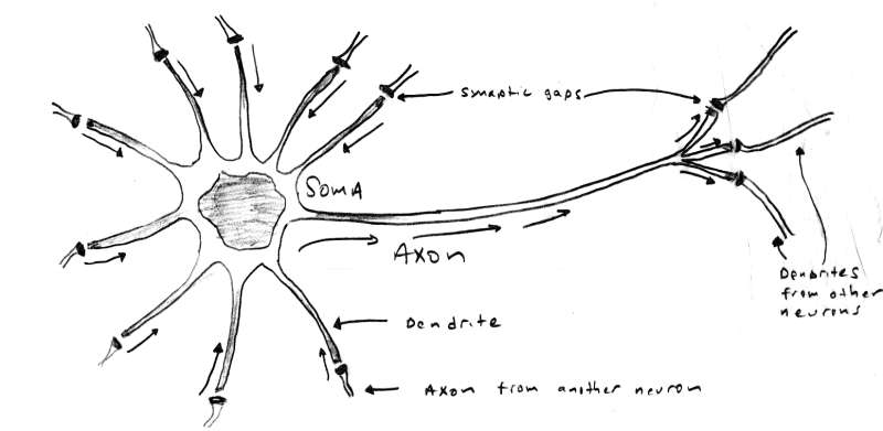
Neural Nets were inspired by our own brains. Literally, some brain in someone's head said, "I wonder how I work?" and then proceeded to create a simple model of itself. Weird huh? The model of the standard neurode is based on a simplified model of a human neuron invented over 50 years ago. Take a look at Figure 1.0. As you can see, there are 3 main parts to a neuron, they are:

• Dendrite(s)........................Responsible for collecting incoming signals.
• Soma................................Responsible for the main processing and summation of signals.
• Axon.................................Responsible for transmitting signals to other dendrites.

[color="#000000"]The average human brain has about 100,000,000,000 or 10[sup]11[/sup] neurons and each neuron has up to 10,000 connections [/color]via the dendrites. The signals are passed via electro-chemical processes based on NA (sodium), K (potassium), and CL (chloride) ions. Signals are transferred by accumulation and potential differences caused by these ions, the chemistry is unimportant, but the signals can be thought of simple electrical impulses that travel from axon to dendrite. The connections from one dendrite to axon are called synapses and these are the basic signal transfer points.

So how does a neuron work? Well, that doesn't have a simple answer, but for our purposes the following explanation will suffice. The dendrites collect the signals received from other neurons, then the soma performs a summation of sorts and based on the result causes the axon to fire and transmit the signal. The firing is contingent upon a number of factors, but we can model it as an transfer function that takes the summed inputs, processes them, and then creates an output if the properties of the transfer function are met. In addition, the output is non-linear in real neurons, that is, signals aren't digital, they are analog. In fact, neurons are constantly receiving and sending signals and the real model of them is frequency dependent and must be analyzed in the S-domain (the frequency domain). The real transfer function of a simple biological neuron has, in fact, been derived and it fills a number of chalkboards up.

Now that we have some idea of what neurons are and what we are trying to model, let's digress for a moment and talk about what we can use neural nets for in video games.


[size="5"]Applications to Games

Neural nets seem to be the answer that we all are looking for. If we could just give the characters in our games a little brains, imagine how cool a game would be! Well, this is possible in a sense. Neural nets model the structure of neurons in a crude way, but not the high level functionality of reason and deduction, at least in the classical sense of the words. It takes a bit of thought to come up with ways to apply neural net technology to game AI, but once you get the hang of it, then you can use it in conjunction with deterministic algorithms, fuzzy logic, and genetic algorithms to create very robust thinking models for your games. Without a doubt better than anything you can do with hundreds of if-then statements or scripted logic. Neural nets can be used for such things as:

Environmental Scanning and Classification - A neural net can be feed with information that could be interpreted as vision or auditory information. This information can then be used to select an output response or teach the net. These responses can be learned in real-time and updated to optimize the response.

Memory - A neural net can be used by game creatures as a form of memory. The neural net can learn through experience a set of responses, then when a new experience occurs, the net can respond with something that is the best guess at what should be done.

Behavioral Control - The output of a neural net can be used to control the actions of a game creature. The inputs can be various variables in the game engine. The net can then control the behavior of the creature.

Response Mapping - Neural nets are really good at "association" which is the mapping of one space to another. Association comes in two flavors: autoassociation which is the mapping of an input with itself and heterassociation which is the mapping of an input with something else. Response mapping uses a neural net at the back end or output to create another layer of indirection in the control or behavior of an object. Basically, we might have a number of control variables, but we only have crisp responses for a number of certain combinations that we can teach the net with. However, using a neural net on the output, we can obtain other responses that are in the same ballpark as our well defined ones.

The above examples may seem a little fuzzy, and they are. The point is that neural nets are tools that we can use in whatever way we like. The key is to use them in cool ways that make our AI programming simpler and make game creatures respond more intelligently.


[size="5"]Neural Nets 101

In this section we're going to cover the basic terminology and concepts used in neural net discussions. This isn't easy since neural nets are really the work of a number of different disciplines, and therefore, each discipline creates their own vocabulary. Alas, the vocabulary that we will learn is a good intersection of all the well know vocabularies and should suffice. In addition, neural network theory is replete with research that is redundant, meaning that many people re-invent the wheel. This has had the effect of creating a number of neural net architectures that have names. I will try to keep things as generic as possible, so that we don't get caught up in naming conventions. Later in the article we will cover some nets that are distinct enough that we will refer to them will their proper names. As you read don't be too alarmed if you don't make the "connections" with all of the concepts, just read them, we will cover most of them again in full context in the remainder of the article. Let's begin... [color="#000088"]

[/color]

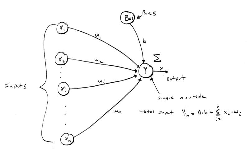
[color="#000088"]Figure 2.0 - A Single Neurode with n Inputs.[/color]

Now that we have seen the wetware version of a neuron, let's take a look at the basic artificial neuron to base our discussions on. Figure 2.0 is a graphic of a standard "neurode" or "artificial neuron". As you can see, it has a number of inputs labeled X[sub]1[/sub] - X[sub]n[/sub] and B. These inputs each have an associated weight w[sub]1[/sub] - w[sub]n[/sub], and b attached to them. In addition, there is a summing junction Y and a single output y. The output y of the neurode is based on a transfer or "activation" function which is a function of the net input to the neurode. The inputs come from the X[sub]i'[/sub]s and from B which is a bias node. Think of B as a "past history", "memory", or "inclination". The basic operation of the neurode is as follows: the inputs X[sub]i[/sub] are each multiplied by their associated weights and summed. The output of the summing is referred to as the input activation Y[sub]a[/sub]. The activation is then fed to the activation function f[sub]a[/sub](x) and the final output is y. The equations for this is:

[/font][/color][color="RED"][font="Symbol"] [/font] X[sub]i[/sub] * w[sub]i[/sub]
[nbsp][nbsp][nbsp][nbsp][nbsp][nbsp][nbsp][nbsp][nbsp][nbsp][nbsp][nbsp][nbsp][nbsp][nbsp][nbsp][nbsp][nbsp][nbsp][nbsp][nbsp]i =1


AND

[/color][color="RED"]y = f[sub]a[/sub](Y[sub]a[/sub]) [/color]

The various forms of f[sub]a[/sub](x) will be covered in a moment.

Before we move on, we need to talk about the inputs X[sub]i[/sub], the weights w[sub]i[/sub], and their respective domains. In most cases, inputs consist of the positive and negative integers in the set ( -[font="Symbol"]?[/font] , +inputs are [font="Symbol"]?[/font] ). However, many neural nets use simpler bivalent values (meaning that they have only two values). The reason for using such a simple input scheme is that ultimately all binary as image or bipolar and complex inputs are converted to pure binary or bipolar representations anyway. In addition, many times we are trying to solve computer problems such or voice recognition which lend themselves to bivalent representations. Nevertheless, this is not etched in stone. In any case, the values used in bivalent systems are primarily 0 and 1 in a binary system or -1 and 1 in a bipolar system. Both systems are similar except that bipolar representations turn out to be mathematically better than binary ones. The weights w[sub]i[/sub] on each input are typically in the range bias ( -? , +? ). and are referred to as excitatory, and inhibitory for positive and negative values respectively. The extra input B which is called the is always 1.0 and is scaled or multiplied by b, that is, b is it's weight in a sense. This is illustrated in Eq.1.0 by the leading term.

Continuing with our analysis, once the activation Y[sub]a[/sub] is found for a neurode then it is applied to the activation function and the output y can be computed. There are a number of activation functions and they have different uses. The basic activation functions f[sub]a[/sub](x) are:

The equations for each are fairly simple, but each are derived to model or fit various properties.

The step function is used in a number of neural nets and models a neuron firing when a critical input signal is reached. This is the purpose of the factor [font="Symbol"]q[/font], it models the critical input level or threshold that the neurode should fire at. The linear activation function is used when we want the output of the neurode to more closely follow the input activation. This kind of activation function would be used in modeling linear systems such as basic motion with constant velocity. Finally, the exponential activation function is used to create a non-linear response which is the only possible way to create neural nets that have non-linear responses and model non-linear processes. The exponential activation function is key in advanced neural nets since the composition of linear and step activation functions will always be linear or step, we will never be able to create a net that has non-linear response, therefore, we need the exponential activation function to address the non-linear problems that we want to solve with neural nets. However, we are not locked into using the exponential function. Hyperbolic, logarithmic, and transcendental functions can be used as well depending on the desired properties of the net. Finally, we can scale and shift all the functions if we need to. [color="#000088"]

[/color]

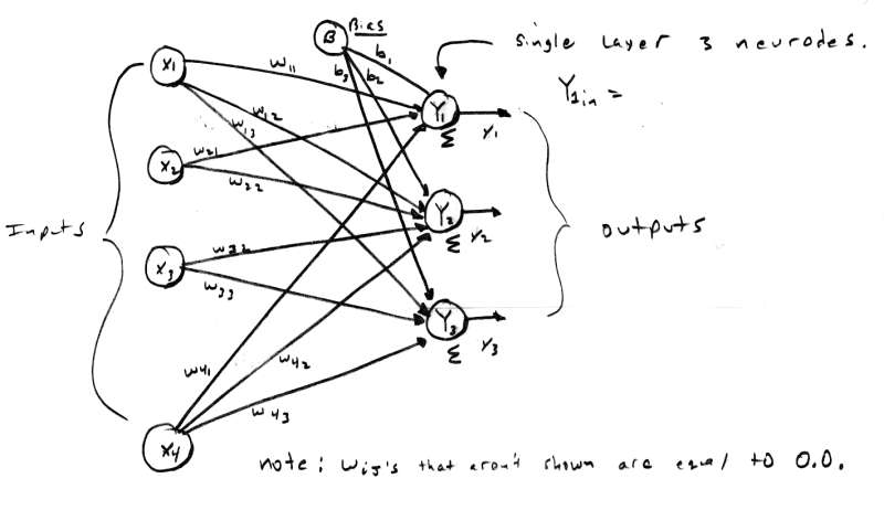
[color="#000088"]Figure 3.0 - A 4 Input, 3 Neurode, SingleLayer Neural Net.[/color][color="#000088"]

[/color]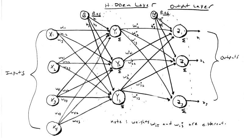
[color="#000088"]Figure 4.0 - A 2 Layer Neural Network.[/color]

As you can imagine, a single neurode isn't going to do a lot for us, so we need to take a group of them and create a layer of neurodes, this is shown in Figure 3.0. The figure illustrates a single layer neural network. The neural net in Figure 3.0 has a number of inputs and a number of output nodes. By convention this is a single layer net since the input layer is not counted unless it is the only layer in the network. In this case, the input layer is also the output layer and hence there is one layer. Figure 4.0 shows a two layer neural net. Notice that the input layer is still not counted and the internal layer is referred to as "hidden". The output layer is referred to as the output or response layer. Theoretically, there is no limit to the number of layers a neural net can have, however, it may be difficult to derive the relationship of the various layers and come up with tractable training methods. The best way to create multilayer neural nets is to make each network one or two layers and then connect them as components or functional blocks.

All right, now let's talk about temporal or time related topics. We all know that our brains are fairly slow compared to a digital computer. In fact, our brains have cycle times in the millisecond range whereas digital computers have cycle times in the nanosecond and soon sub-nanosecond times. This means that signals take time to travel from neuron to neuron. This is also modeled by artificial neurons in the sense that we perform the computations layer by layer and transmit the results sequentially. This helps to better model the time lag involved in the signal transmission in biological systems such as us.

We are almost done with the preliminaries, let's talk about some high level concepts and then finish up with a couple more terms. The question that you should be asking is, "what the heck to neural nets do?" This is a good question, and it's a hard one to answer definitively. The question is more, "what do you want to try and make them do?" They are basically mapping devices that help map one space to another space. In essence, they are a type of memory. And like any memory we can use some familiar terms to describe them. Neural nets have both STM (Short Term Memory) and LTM (Long Term Memory). STM is the ability for a neural net to remember something it just learned, whereas, LTM is the ability of a neural net to remember something it learned some time ago amongst its new learning. This leads us to the concepts of plasticity or in other words how a neural net deals with new information or training. Can a neural net learn more information and still recall previously stored information correctly? If so, does the neural net become unstable since it is holding so much information that the data starts to overlapping or has common intersections. This is referred to as stability. The bottom line is we want a neural net to have a good LTM, a good STM, be plastic (in most cases) and exhibit stability. Of course, some neural nets have no analog to memory they are more for functional mapping, so these concepts don't apply as is, but you get the idea. Now that we know about the aforementioned concepts relating to memory, let's finish up by talking some of the mathematical factors that help measure and understand these properties.

One of the main uses for neural nets are memories that can process input that is either incomplete or noisy and return a response. The response may be the input itself (autoassociation) or another output that is totally different from the input (heteroassociation). Also, the mapping may be from a n-dimensional space to a m-dimensional space and non-linear to boot. The bottom line is that we want to some how store information in the neural net so that inputs (perfect as well as noisy) can be processed in parallel. This means that a neural net is a kind of hyperdimensional memory unit since it can associate an input n-tuple with an output m-tupple where m can equal n, but doesn't have to.

What neural nets do in essence is partition an n-dimensional space into regions that uniquely map the input to the output or classify the input into distinct classes like a funnel of sorts. Now, as the number of input values (vectors) in the input data set increase which we will refer to as S, it logically follows that the neural net is going to have harder time separating the information. And as a neural net is filled with information, the input values that are to be recalled will overlap since the input space can no longer keep everything partitioned in a finite number of dimensions. This overlap results in crosstalk, meaning that some inputs are not as distinct as they could be. This may or may not be desired. Although this problem isn't a concern in all cases, it is a concern in associative memory neural nets, so to illustrate the concept let's assume that we are trying to associate n-tuple input vectors with some output set. The output set isn't as much of a concern to proper functioning as is the input set S is.

If a set of inputs S is straight binary then we are looking at sequences in the form 1101010...10110 let's say that our input bit vectors are only 3 bits each, therefore the entire input space consist of the vectors:

To be more precise the Basis for this set of vectors is:

For example if we let b[sub]2[/sub]=1, b[sub]1[/sub]=0, and b[sub]0[/sub]=1 then we get the vector:

A basis is a special vector summation that describes a set of vectors in a space. So v describes all the vector in our space. Now to make a long story short, the more orthogonal the vectors in the input set are the better they will distribute in a neural net and the better they can be recalled. Orthogonality refers to the independence of the vectors or in other words if two vector are orthogonal then their dot product is 0, their projection onto one another is 0, and they can't be written in terms of one another. In the set v there are a lot of orthogonal vectors, but they come in small groups, for example v[sub]0[/sub] is orthogonal to all the vectors, so we can always include it. But if we include v[sub]1[/sub] in our set S then the only other vectors that will fit and maintain orthogonality are v[sub]2[/sub] and v[sub]4[/sub] or the set:

Why? Because v[sub]i[/sub] [font="Symbol"]+[/font] v[sub]j[/sub] for all i,j from 0..3 is equal to 0. In other words, the dot product of all the pairs of vectors in 0, so they must all be orthogonal. Therefore, this set will do very well in a neural net as input vectors. However, the set:

will potentially do poorly as inputs since v[sub]6[/sub][font="Symbol"]+[/font]v[sub]7[/sub] is non-zero or in a binary system it is 1. The next question is, "can we measure this orthogonality?" The answer is yes. In the binary vector system there is a measure called hamming distance. It is used to measure the n-dimensional distance between binary bit vectors. It is simply, the number of bits that are different between two vectors. For example the vectors:

have a hamming distance of 1 while the vectors,

have a hamming distance of 2.

We can use hamming distance as the measure of orthogonality in binary bit vector systems. And this can help us determine if our input vectors are going to have a lot of overlap. Determining orthogonality with general vector inputs is harder, but the concept is the same. That's all the time we have for concepts and terminology, so let's jump right in and see some actual neural nets that do something and hopefully by the end of the article you will be able to use them in your game's AI. We are going to cover neural nets used to perform logic functions, classify inputs, and associate inputs with outputs. [color="#000088"]

[/color]

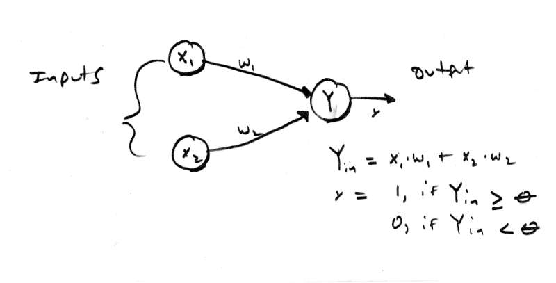
[color="#000088"]Figure 5.0 - The McCulloch-Pitts Neurode.[/color]

[size="5"]Pure Logic Mr. Spock

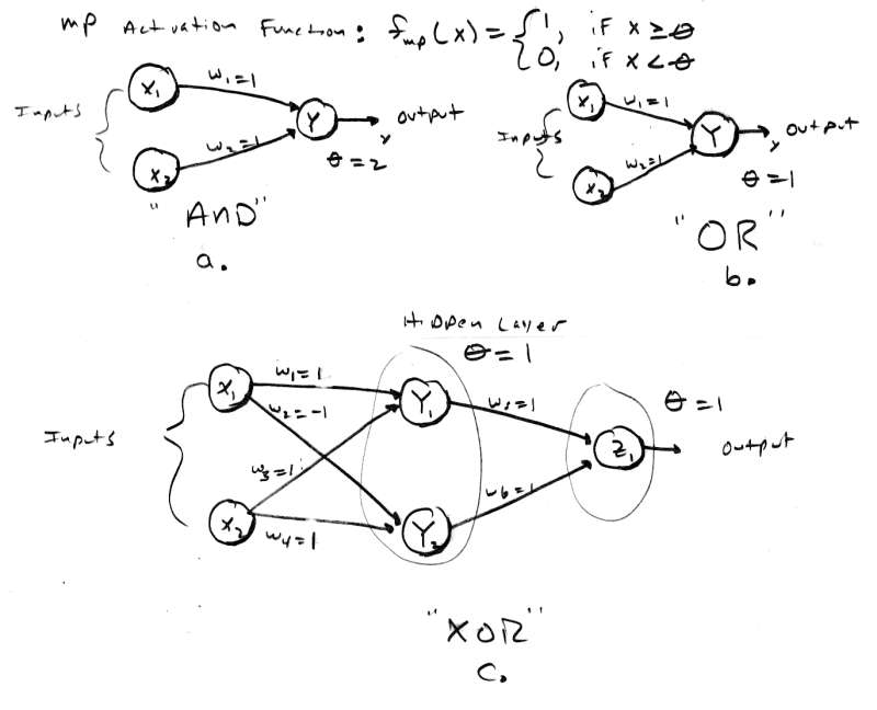
The first artificial neural networks were created in 1943 by McCulloch and Pitts. The neural networks were composed of a number of neurodes and were typically used to compute simple logic functions such as AND, OR, XOR, and combinations of them. Figure 5.0 is a representation of a basic McCulloch-Pitts neurode with 2 inputs. If you are an electrical engineer then you will immediately see a close resemblance between McCulloch-Pitts neurodes and transistors or MOSFETs. In any case, McCulloch-Pitts neurodes do not have biases and have the simple activation function f[sub]mp[/sub](x) equal to:

The MP (McCulloch-Pitts) neurode functions by summing the product of the inputs X[sub]i[/sub] and weights w[sub]i[/sub] and applying the result Y[sub]a[/sub] to the activation function f[sub]mp[/sub](x). The early research of McCulloch-Pitts focused on creating complex logical circuitry with the neurode models. In addition, one of the rules of the neurode model is that is takes one time step for a signal to travel from neurode to neurode. This helps model the biological nature of neurons more closely. Let's take a look at some examples of MP neural nets that implement basic logic functions. The logical AND function has the following truth table:

X1X2Output000010100111[color="#000088"]Table 1.0 - Truth Table for Logical[/color][color="#000088"] AND.

[/color]

[color="#000088"]Figure 6.0 - Basic Logic Functions Implemented with McCulloch-Pitts Nets.[/color]

We can model this with a two input MP neural net with weights w[sub]1[/sub]=1, w[sub]2[/sub]=1, and [font="Symbol"]q[/font] = 2. This neural net is shown in Figure 6.0a. As you can see, all input combinations work correctly. For example, if we try inputs X[sub]1[/sub]=0, Y[sub]1[/sub]=1, then the activation will be:

If we apply 1.0 to the activation function f[sub]mp[/sub](x) then the result is 0 which is correct. As another example, if we try inputs X[sub]1[/sub]=1, X[sub]2[/sub]=1, then the activation will be:

If we input 2.0 to the activation function f[sub]mp[/sub](x), then the result is 1.0 which is correct. The other cases will work also. The function of the OR is similar, but the threshold [font="Symbol"]q[/font] of is changed to 1.0 instead 2.0 as it is in the AND. You can try running through the truth table yourself to see the results.

The XOR network is a little different because it really has 2 layers in a sense because the results of the pre-processing are further processed in the output neuron. This is a good example of why a neural net needs more than one layer to solve certain problems. The XOR is a common problem in neural nets that is used to test a neural net's performance. In any case, XOR is not linearly separable in a single layer, it must be broken down into smaller problems and then the results added together. Let's take a look at XOR as the final example of MP neural networks. The truth table for XOR is as follows: [color="#000088"]

[color="#000000"]X1 X2Output000011101110[/color]Table 2.0 - Truth Table for Logical XOR.

[/color]

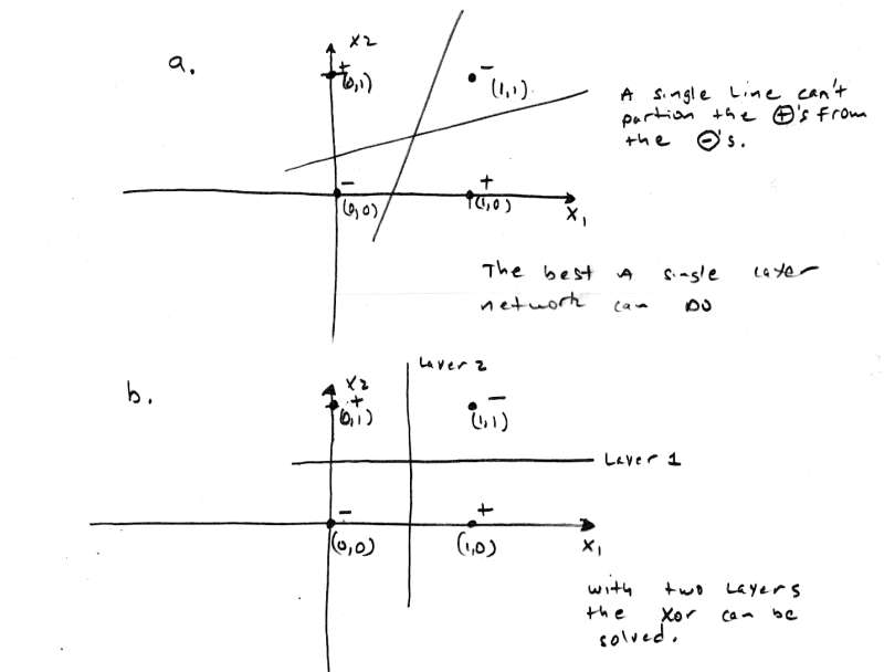
[color="#000088"]Figure 7.0 - Using the XOR Function to Illustrate Linear Separability.[/color]

XOR is only true when the inputs are different, this is a problem since both inputs map to the same output. XOR is not linearly separable, this is shown in Figure 7.0. As you can see, there is no way to separate the proper responses with a straight line. The point is that we can separate the proper responses with 2 lines and this is just what 2 layers do. The first layer pre-processes or solves part of the problem and the remaining layer finishes up. Referring to Figure 6.0c, we see that the weights are w[sub]1[/sub]=1, w[sub]2[/sub]=-1, w[sub]3[/sub]=1, w[sub]4[/sub]=-1, w[sub]5[/sub]=1, w[sub]6[/sub]=1. The network works as follows: layer one computes if X[sub]1[/sub] and X[sub]2[/sub] are opposites in parallel, the results of either case (0,1) or (1,0) are feed to layer two which sums these up and fires if either is true. In essence we have created the logic function:

If you would like to experiment with the basic McCulloch Pitts neurode Listing 1.0 is a complete 2 input, single neurode simulator that you can experiment with.

That finishes up our discussion of the basic building block invented by McCulloch and Pitts now let's move on to more contemporary neural nets such as those used to classify input vectors.
[color="#000088"]
[/color]

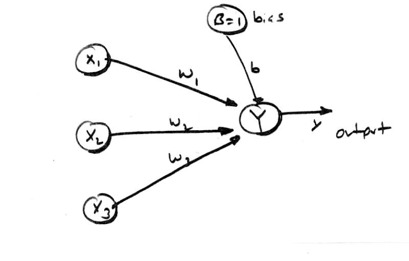
[color="#000088"]Figure 8.0 - The Basic Neural Net Model Used for Discussion.[/color]

[size="5"]Classification and "Image" Recognition

At this point we are ready to start looking at real neural nets that have some girth to them! To segue into the following discussions on Hebbian, and Hopfield neural nets, we are going to analyze a generic neural net structure that will illustrate a number of concepts such as linear separability, bipolar representations, and the analog that neural nets have with memories. Let's begin with taking a look at Figure 8.0 which is the basic neural net model we are going to use. As you can see, it is a single node net with 3 inputs including the bias, and a single output. We are going to see if we can use this network to solve the logical AND function that we solved so easily with McCulloch-Pitts neurodes.

Let's start by first using bipolar representations, so all 0's are replaced with -1's and 1's are left alone. The truth table for logical AND using bipolar inputs and outputs is shown below: [color="#000088"]

[color="#000000"]X1X2Output-1-1-1-11-11-1-1111[/color]Table 3.0 - Truth Table for Logical AND in Bipolar Format.[/color]

And here is the activation function f[sub]c[/sub](x) that we will use:

Notice that the function is step with bipolar outputs. Before we continue, let me place a seed in your mind; the bias and threshold end up doing the same thing, they give us another degree of freedom in our neurons that make the neurons respond in ways that can't be achieved without them. You will see this shortly.

The single neurode net in Figure 8.0 is going to perform a classification for us. It is going to tell us if our input is in one class or another. For example, is this image a tree or not a tree. Or in our case is this input (which just happens to be the logic for an AND) in the +1 or -1 class? This is the basis of most neural nets and the reason I was belaboring linear separability. We need to come up with a linear partitioning of space that maps our inputs and outputs so that there is a solid delineation of space that separates them. Thus, we need to come up with the correct weights and a bias that will do this for us. But how do we do this? Do we just use trial and error or is there a methodology? The answer is that there are a number of training methods to teach a neural net. These training methods work on various mathematical premises and can be proven, but for now, we're just going to pull some values out of the hat that work. These exercises will lead us into the learning algorithms and more complex nets that follow.

All right, we are trying to finds weights w[sub]i[/sub] and bias b that give use the correct result when the various inputs are feed to our network with the given activation function f[sub]c[/sub](x). Let's write down the activation summation of our neurode and see if we can infer any relationship between the weights and the inputs that might help us. Given the inputs X[sub]1[/sub] and X[sub]2[/sub] with weights w[sub]1[/sub] and w[sub]2[/sub] along with B=1 and bias b, we have the following formula:

Since B is always equal to 1.0 the equation simplifies to:

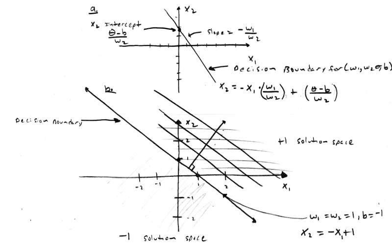
[color="#000088"]Figure 9.0 - Mathematical Decision Boundaries Generated by Weights, Bias, and [font="Symbol"]q[/font][/color]

What is this entity? It's a line! And if the left hand side is greater than or equal to [font="Symbol"]q[/font], that is, (X[sub]1[/sub]*w[sub]1[/sub] + X[sub]2[/sub]*w[sub]2[/sub] + b) then the neurode will fire and output 1, otherwise the neurode will output -1. So the line is a decision boundary. Figure 9.0a illustrates this. Referring to the figure, you can see that the slope of the line is -w[sub]1[/sub]/w[sub]2[/sub] and the X[sub]2[/sub] intercept is ([font="Symbol"]q[/font] -b)/w[sub]2[/sub]. Now can you see why we can get rid of [font="Symbol"]q[/font]? It is part of a constant and we can always scale b to take up any loss, so we will assume that [font="Symbol"]q[/font] = 0, and the resulting equation is:

What we want to find are weights w[sub]1[/sub] and w[sub]2[/sub] and bias b so that it separates our outputs or classifies them into singular partitions without overlap. This is the key to linear separability. Figure 9.0b shows a number of decision boundaries that will suffice, so we can pick any of them. Let's pick the simplest values which would be:

With these values our decision boundary becomes:

The slope is -1 and the X[sub]2[/sub] intercept is 1. If we plug the input vectors for the logical AND into this equation and use the f[sub]c[/sub](x) activation function then we will get the correct outputs. For example if, X[sub]2[/sub] + X[sub]1[/sub]-1 >0 then fire the neurode, else output -1. Let's try it with our AND inputs and see what we come up with: [color="#000088"]

Input X1X2Output (X2+X1-1) -1-1(-1) +( -1) -1 = 3 < 0 don't fire, output -1 -11(-1) + (1) -1 = -1< 0 don't fire, output -1 1-1(1) + (-1) -1 = -2 < 0 don't fire, output -1 11(1) + (1)-1 = 1 > 0 fire, output 1Table 4.0 - Truth Table for Bipolar AND with decision boundary.[/color]

As you can see, the neural network with the proper weights and bias solves the problem perfectly. Moreover, there are a whole family of weights that will do just as well (sliding the decision boundary in a direction perpendicular to itself). However, there is an important point here. Without the bias or threshold, only lines through the origin would be possible since the X[sub]2[/sub] intercept would have to be 0. This is very important and the basis for using a bias or threshold, so this example has proven to be an important one since it has flushed this fact out. So, are we closer to seeing how to algorithmically find weights? Yes, we now have a geometrical analogy and this is the beginning of finding an algorithm.


[size="5"]The Ebb of Hebbian

Now we are ready to see the first learning algorithm and its application to a neural net. One of the simplest learning algorithms was invented by Donald Hebb and it is based on using the input vectors to modify the weights in a way so that the weight create the best possible linear separation of the inputs and outputs. Alas, the algorithm works just OK. Actually, for inputs that are orthogonal it is perfect, but for non-orthogonal inputs, the algorithm falls apart. Even though, the algorithm doesn't result in correct weight for all inputs, it is the basis of most learning algorithms, so we will start here.

Before we see the algorithm, remember that it is for a single neurode, single layer neural net. You can of course, place a number of neurodes in the layer, but they will all work in parallel and can be taught in parallel. Are you starting to see the massive parallization that neural nets exhibit? Instead of using a single weight vector, a multi-neurode net uses a weight matrix. Anyway, the algorithm is simple, it goes something like this:

[/color] Step 1. Initialize all your weights to 0, and let them be contained in a vector w that has n entries. Also initialize the bias b to 0.

Step 2. For j = 1 to n do

end do

The algorithm is nothing more than an "accumulator" of sorts. Shifting, the decision boundary based on the changes in the input and output. The only problem is that it sometimes can't move the boundary fast enough (or at all) and "learning" doesn't take place.

So how do we use Hebbian learning? The answer is, the same as the previous network except that now we have an algorithmic method teach the net with, thus we refer to the net as a Hebb or Hebbian Net. As an example, let's take our trusty logical AND function and see if the algorithm can find the proper weights and bias to solve the problem. The following summation is equivalent to running the algorithm:

Therefore, w[sub]1[/sub]=2, w[sub]2[/sub]=2, and b=-2. These are simply scaled versions of the values w[sub]1[/sub]=1, w[sub]2[/sub]=1, b=-1 that we derived geometrically in the previous section. Killer huh! With this simple learning algorithm we can train a neural net (consisting of a single neurode) to respond to a set of inputs and either classify the input as true or false, 1 or -1. Now if we were to array these neurodes together to create a network of neurodes then instead of simple classifying the inputs as on or off, we can associate patterns with the inputs. This is one of the foundations for the next network neural net structure; the Hopfield net. One more thing, the activation function used for a Hebb Net is a step with a threshold of 0.0 and bipolar outputs 1 and -1.

To get a feel for Hebbian learning and how to implement an actual Hebb Net, Listing 2.0 contains a complete Hebbian Neural Net Simulator. You can create networks with up to 16 inputs and 16 neurodes (outputs). The program is self explanatory, but there are a couple of interesting properties: you can select 1 of 3 activation functions, and you can input any kind of data you wish. Normally, we would stick to the Step activation function and inputs/outputs would be binary or bipolar. However, in the light of discovery, maybe you will find something interesting with these added degrees of freedom. However, I suggest that you begin with the step function and all bipolar inputs and outputs.



[size="5"]Playing the Hopfield[color="#000088"]

[/color]

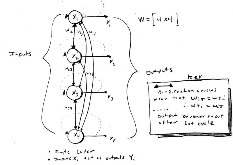
[color="#000088"]Figure 10.0 - A 4 Node Hopfield Autoassociative Neural Net.[/color]

John Hopfield is a physicist that likes to play with neural nets (which is good for us). He came up with a simple (in structure at least), but effective neural network called the Hopfield Net. It is used for autoassociation, you input a vector x and you get x back (hopefully). A Hopfield net is shown in Figure 10.0. It is a single layer network with a number of neurodes equal to the number of inputs X[sub]i[/sub]. The network is fully connected meaning that every neurode is connected to every other neurode and the inputs are also the outputs. This should strike you as weird since there is feedback. Feedback is one of the key features of the Hopfield net and this feedback is the basis for the convergence to the correct result.

The Hopfield network is an iterative autoassociative memory. This means that is may take one or more cycles to return the correct result (if at all). Let me clarify; the Hopfield network takes an input and then feeds it back, the resulting output may or may not be the desired input. This feedback cycle may occur a number of times before the input vector is returned. Hence, a Hopfield network functional sequence is: first we determine the weights based on our input vectors that we want to autoassociate, then we input a vector and see what comes out of the activations. If the result is the same as our original input then we are done, if not, then we take the result vector and feed it back through the network. Now let's take a look at the weight matrix and learning algorithm used for Hopfield nets.

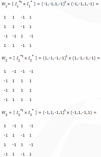
The learning algorithm for Hopfield nets is based on the Hebbian rule and is simply a summation of products. However, since the Hopfield network has a number of input neurons the weights are no longer a single array or vector, but a collection of vectors which are most compactly contained in a single matrix. Thus the weight matrix W for a Hopfield net is created based on this equation:

[color="#000088"]Eq. 8.0[/color]

[/color][color="RED"][nbsp][nbsp][nbsp][nbsp][nbsp][nbsp][nbsp][nbsp][nbsp][nbsp][nbsp][nbsp][nbsp][nbsp][nbsp][nbsp][nbsp][nbsp][nbsp]k
W [sub](kxk)[/sub] = [/color][color="RED"][font="Symbol"]?[/font][/color][color="RED"] I[sub]i[/sub][sup]t[/sup] x I[sub]i[/sub]
[nbsp][nbsp][nbsp][nbsp][nbsp][nbsp][nbsp][nbsp][nbsp][nbsp][nbsp][nbsp][nbsp][nbsp][nbsp][nbsp][nbsp][nbsp][nbsp]i = 1
[/color]

note: each outer product will have dimension k x k, since we are multiplying a column vector and a row vector.

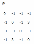
and, W[sub]ii[/sub] = 0, for all i.

Notice that there are no bias terms and the main diagonal of W must be all zero's. The weight matrix is simply the sum of matrices generated by multiplying the transpose I[sub]i[/sub][sup]t[/sup] x I[sub]i [/sub]for all i from 1 to n. This is almost identical to the Hebbian algorithm for a single neurode except that instead of multiplying the input by the output, the input is multiplied by itself, which is equivalent to the output in the case of autoassociation. Finally, the activation function f[sub]h[/sub](x) is shown below:

f[sub]h[/sub](x) it is a step function with a binary output. This means that the inputs must be binary, but we already said that inputs are bipolar? Well, they are, and they aren't. When the weight matrix is generated we convert all input vectors to bipolar, but for normal operation we use the binary version of the inputs and the output of the Hopfield net will also be binary. This convention is not necessary, but makes the network discussion a little simpler. Anyway, let's move on to an example. Say we want to create a four node Hopfield net and we want it to recall these vectors:

Converting to bipolar *, we have:

Now we need to compute W[sub]1[/sub], W[sub]2[/sub], W[sub]3[/sub], where W[sub]i[/sub] is the product of the transpose of each input with itself.



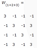
Then we add W[sub]1[/sub] + W[sub]2[/sub] + W[sub]3[/sub] resulting in:



Zeroing out the main diagonal gives us the final weight matrix:



That's it, now we are ready to rock. Let's input our original vectors and see the results. To do this we simply have to matrix multiple the input by the matrix and then process each output value with our activation function f[sub]h[/sub](x). Here are the results:

The inputs were perfectly recalled, and they should be since they were all orthogonal. As a final example, let's assume that our input (vision, auditory etc.) is a little noisy and the input has a single error in it. Let's take I[sub]3[/sub] = (0,1,0,1) and add some noise to I[sub]3[/sub] resulting in I[sub]3[/sub][sup]noise[/sup] = (0,1,1,1). Now let's see what happens if we input this noisy vector to the Hopfield net:

Amazingly enough, the original vector is recalled. This is very cool. So we might have a memory that is filled with bit patterns that look like trees, (oaks, weeping willow, spruce, redwood etc.) then if we input another tree that is similar to say a weeping willow, but hasn't been entered into the net, our net will (hopefully) output a weeping willow indicating that this is what it "thinks" it looks like. This is one of the strengths of associative memories, we don't have to teach it every possible input, but just enough to give it a good idea. Then inputs that are "close" will usually converge to an actual trained input. This is the basis for image, and voice recognition systems. Don't ask me where the heck the "tree" analogy came from. Anyway, to complete our study of neural nets, I have included a final Hopfield autoassociative simulator that allows you to create nets with up to 16 neurodes. It is similar to the Hebb Net, but you must use a step activation function and your inputs exemplars must be in bipolar while training and binary while associating (running). Listing 3.0 contains the code for the simulator.



[size="5"]Brain Dead...

Well that's all we have time for. I was hoping to get to the Perceptron network, but oh well. I hope that you have an idea of what neural nets are and how to create some working computer programs to model them. We covered basic terminology and concepts, some mathematical foundations, and finished up with some of the more prevalent neural net structures. However, there is still so much more to learn about neural nets. We need to cover Perceptrons, Fuzzy Associative Memories or FAMs, Bidirectional Associative Memories or BAMs, Kohonen Maps, Adalines, Madalines, Backpropagation networks, Adaptive Resonance Theory networks, "Brain State in a Box", and a lot more. Well that's it, my neural net wants to play N64!