The Total Beginner's Guide to Game AI

Programming

Artificial Intelligence

Published August 13, 2018 by Ben Sizer, posted by Kylotan

Do you see issues with this article? Let us know.

Introduction

This article will introduce you to a range of introductory concepts used in artificial intelligence for games (or ‘Game AI’ for short) so that you can understand what tools are available for approaching your AI problems, how they work together, and how you might start to implement them in the language or engine of your choice.

We’re going to assume you have a basic knowledge of video games, and some grasp on mathematical concepts like geometry, trigonometry, etc. Most code examples will be in pseudo-code, so no specific programming language knowledge should be required.

What is Game AI?

Game AI is mostly focused on which actions an entity should take, based on the current conditions. This is what the traditional AI literature refers to as controlling ‘intelligent agents’ where the agent is usually a character in the game – but could also be a vehicle, a robot, or occasionally something more abstract such as a whole group of entities, or even a country or civilization. In each case it is a thing that needs to observe its surroundings, make decisions based on that, and act upon them. This is sometimes thought of as the Sense/Think/Act cycle:

Sense: The agent detects - or is told about - things in their environment that may influence their behaviour (e.g. threats nearby, items to collect, points of interest to investigate)
Think: The agent makes a decision about what to do in response (e.g. considers whether it is safe enough to collect items, or whether it should focus on fighting or hiding first)
Act: The agent performs actions to put the previous decision into motion (e.g. starts moving along a path towards the enemy, or towards the item, etc)
...the situation has now changed, due to the actions of the characters, so the cycle must repeat with the new data.

In real-world AI problems, especially the ones making the news at the moment, they are typically heavily focused on the ‘sense’ part of this cycle. For example, autonomous cars must take images of the road ahead, combine them with other data such as radar and LIDAR, and attempt to interpret what they see. This is usually done by some sort of machine learning, which is especially good at taking a lot of noisy, real-world data (like a photo of the road in front of a car, or a few frames of video) and making some sense of that, extracting semantic information such as “there is another car 20 yards ahead of you”. These are referred to as ‘classification problems’.

Games are unusual in that they don’t tend to need a complex system to extract this information, as much of it is intrinsic to the simulation. There’s no need to run image recognition algorithms to spot if there’s an enemy ahead; the game knows there is an enemy there and can feed that information directly in to the decision making process. So the ‘sense’ part of the cycle is often much simpler, and the complexity arises in the ‘think’ and ‘act’ implementations.

Constraints of Game AI development

AI for games usually has a few constraints it has to respect:

It isn’t usually ‘pre-trained’ like a machine learning algorithm would be; it’s not practical to write a neural network during development to observe tens of thousands of players and learn the best way to play against them, because the game isn’t released yet and there are no players!
The game is usually supposed to provide entertainment and challenge rather than be ‘optimal’ - so even if the agents could be trained to take the best approach against the humans, this is often not what the designers actually want.
There is often a requirement for agents to appear ‘realistic’, so that players can feel that they’re competing against human-like opponents. The AlphaGo program was able to become far better than humans but the moves chosen were so far from the traditional understanding of the game that experienced opponents would say that it “almost felt like I was playing against an alien”. If a game is simulating a human opponent, this is typically undesirable, so the algorithm would have to be tweaked to make believable decisions rather than the ideal ones.
It needs to run in ‘real-time’, which in this context means that the algorithm can’t monopolise CPU usage for a long time in order to make the decision. Even taking just 10 milliseconds to make a decision is far too long because most games only have somewhere between 16 and 33 milliseconds to perform all the processing for the next frame of graphics.
It’s ideal if at least some of the system is data-driven rather than hard-coded, so that non-coders can make adjustments, and so that adjustments can be made more quickly.

With that in mind, we can start to look at some extremely simple AI approaches that cover the whole Sense/Think/Act cycle in ways that are efficient and allow the game designers to choose challenging and human-like behaviours.

Basic Decision Making

Let’s start with a very simple game like Pong. The aim to move the ‘paddle’ so that the ball bounces off it instead of going past it, the rules being much like tennis in that you lose when you fail to return the ball. The AI has the relatively simple task of deciding which direction to move the paddle.

Hardcoded conditional statements

If we wanted to write AI to control the paddle, there is an intuitive and easy solution – simply try and position the paddle below the ball at all times. By the time the ball reaches the paddle, the paddle is ideally already in place and can return the ball.

A simple algorithm for this, expressed in ‘pseudocode’ below, might be:


every frame/update while the game is running:

if the ball is to the left of the paddle:

	move the paddle left

else if the ball is to the right of the paddle:

	move the paddle right

Providing that the paddle can move at least as fast as the ball does, this should be a perfect algorithm for an AI player of Pong. In cases where there isn’t a lot of sensory data to work with and there aren’t many different actions the agent can perform, you don’t need anything much more complex than this.

This approach is so simple that the whole Sense/Think/Act cycle is barely visible. But it is there.

The ‘sense’ part is in the 2 “if” statements. The game knows where the ball is, and where the paddle is. So the AI asks the game for those positions, and thereby ‘senses’ whether the ball is to the left or to the right.
The ‘think’ part is also built in to the two “if” statements. These embody 2 decisions, which in this case are mutually exclusive, and result in one of three actions being chosen – either to move the paddle left, to move it right, or to do nothing if the paddle is already correctly positioned.
The ‘act’ part is the “move the paddle left” and “move the paddle right” statements. Depending on the way the game is implemented, this might take the form of immediately moving the paddle position, or it might involve setting the paddle’s speed and direction so that it gets moved properly elsewhere in the game code.

Approaches like this are often termed “reactive” because there are a simple set of rules – in this case, ‘if’ statements in the code – which react to the current state of the world and immediately make a decision on how to act.

Decision Trees

This Pong example is actually equivalent to a formal AI concept called a ‘decision tree’. This is a system where the decisions are arranged into a tree shape and the algorithm must traverse it in order to reach a ‘leaf’ which contains the final decision on which action to take. Let’s draw a visual representation of a decision tree for the Pong paddle algorithm, using a flowchart:

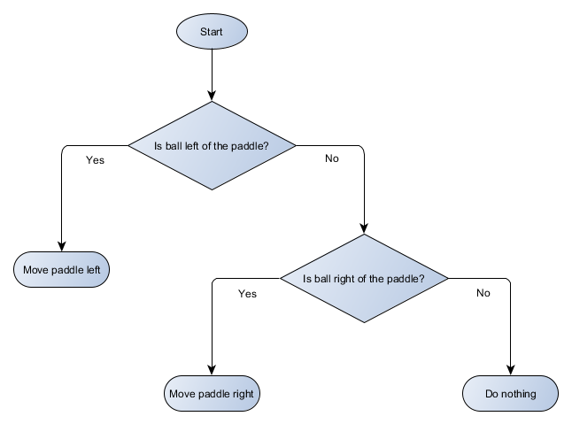
You can see that it it resembles a tree, although an upside-down one!

Each part of the decision tree is typically called a ‘node’ because AI uses graph theory to describe structures like this. Each node is one of two types:

Decision Nodes: a choice between 2 alternatives based on checking some condition, each alternative represented as its own node;
End Nodes: an action to take, which represents the final decision made by the tree.

The algorithm starts at the first node, designated the ‘root’ of the tree, and either takes a decision on which child node to move to based on the condition in the doe, or executes the action stored in the node and stops.

At first glance, it might not be obvious what the benefit is here, because the decision tree is obviously doing the same job as the if-statements in the previous section. But there is a very generic system here, where each decision has precisely 1 condition and 2 possible outcomes, which allows a developer to build up the AI from data that represents the decisions in the tree, avoiding hardcoding it. It’s easy to imagine a simple data format to describe the tree like this:

Node number

Decision (or ‘End’)

Action

Is Ball Left Of Paddle?

Yes? Check Node 2

No? Check Node 3

End

Move Paddle Left

Is Ball Right Of Paddle?

Yes? Goto Node4

No? Goto Node5

End

Move Paddle Right

End

Do Nothing

On the code side, you’d have a system to read in each of these lines, create a node for each one, hook up the decision logic based on the 2nd column, and hook up the child nodes based on the 3rd and 4th columns. You still need to hard-code the conditions and the actions, but now you can imagine a more complex game where you add extra decisions and actions and can tweak the whole AI just by editing the text file with the tree definition in. You could hand the file over to a game designer who can tweak the behaviour without needing to recompile the game and change the code – providing you have provided useful conditions and actions in the code already.

Where decision trees can be really powerful is when they can be constructed automatically based on a large set of examples (e.g. using the ID3 algorithm). This makes them an effective and highly-performant tool to classify situations based on the input data, but this is beyond the scope of a simple designer-authored system for having agents choose actions.

Scripting

Earlier we had a decision tree system that made use of pre-authored conditions and actions. The person designing the AI could arrange the tree however they wanted, but they had to rely on the programmer having already provided all the necessary conditions and actions they needed. What if we could give the designer better tools which allowed them to create some of their own conditions, and maybe even some of their own actions?

For example, instead of the coder having to write code for the conditions “Is Ball Left Of Paddle” and “Is Ball Right Of Paddle”, he or she could just provide a system where the designer writes the conditions to check those values for themself. The decision tree data might end up looking more like this:

Node number

Decision (or ‘End’)

Action

ball.position.x < paddle.position.x

Yes? Check Node 2

No? Check Node 3

End

Move Paddle Left

ball.position.x > paddle.position.x

Yes? Check Node4

No? Check Node5

End

Move Paddle Right

End

Do Nothing

This is the same as above, but the decisions have their own code in them, looking a bit like the conditional part of an if-statement. On the code side, this would read in that 2nd column for the Decision nodes, and instead of looking up the specific condition to run (like “Is Ball Left Of Paddle”), it evaluates the conditional expression and returns true or false accordingly. This can be done by embedding a scripting language, like Lua or Angelscript, which allows the developer to take objects in their game (e.g. the ball and the paddle) and create variables which can be accessed in script (e.g. “ball.position”). The scripting language is usually easier to write than C++ and doesn’t require a full compilation stage, so it’s very suitable for making quick adjustments to game logic and allowing less technical members of the team to be able to shape features without requiring a coder’s intervention.

In the above example the scripting language is only being used to evaluate the conditional expression, but there’s no reason the output actions couldn’t be scripted too. For example, the action data like “Move Paddle Right” could become a script statement like “ball.position.x += 10”, so that the action is also defined in the script, without the programmer needing to hard code a MovePaddleRight function.

Going one step further, it’s possible (and common) to take this to the logical conclusion of writing the whole decision tree in the scripting language instead of as a list of lines of data. This would be code that looks much like the original hardcoded conditional statements we introduced above, except now they wouldn’t be ‘hardcoded’ - they’d exist in external script files, meaning they can be changed without recompiling the whole program. It is often even possible to change the script file while the game is running, allowing developers to rapidly test different AI approaches.

Responding to events

The examples above were designed to run every frame in a simple game like Pong. The idea is that they can continuously run the Sense/Think/Act loop and keep acting based on the latest world state. But with more complex games, rather than evaluating everything, it often makes more sense to respond to ‘events’, which are notable changes in the game environment.

This doesn’t apply so much to Pong, so let’s pick a different example. Imagine a shooter game where the enemies are stationary until they detect the player, and then take different actions based on who they are – the brawlers might charge towards the player, while the snipers will stay back and aim a shot. This is still essentially a basic reactive system – “if player is seen, then do something” - but it can logically be divided up into the event (“Player Seen”), and the reaction (choose a response and carry it out).

This brings us right back to our Sense/Think/Act cycle. We might have a bit of code which is the ‘Sense’ code, and that checks, every frame, whether the enemy can see the player. If not, nothing happens. But if so, it creates the ‘Player Seen’ event. The code would have a separate section which says “When ‘Player Seen’ event occurs, do <xyz>” and the <xyz> is whichever response you need to handle the Thinking and Acting. On your Brawler character, you might hook up your “ChargeAndAttack” response function to the Player Seen event – and on the Sniper character, you would hook up your “HideAndSnipe” response function to that event. As with the previous examples, you can make these associations in a data file so that they can be quickly changed without rebuilding the engine. And it’s also possible (and common) to write these response functions in a scripting language, so that the designers can make complex decisions when these events occur.

Advanced Decision Making

Although simple reactive systems are very powerful, there are many situations where they are not really enough. Sometimes we want to make different decisions based on what the agent is currently doing, and representing that as a condition is unwieldy. Sometimes there are just too many conditions to effectively represent them in a decision tree or a script. Sometimes we need to think ahead and estimate how the situation will change before deciding our next move. For these problems, we need more complex solutions.

Finite state machines

A finite state machine (or FSM for short) is a fancy way of saying that some object – for example, one of our AI agents – is currently in one of several possible states, and that they can move from one state to another. There are a finite number of those states, hence the name. A real-life example is a set of traffic lights, which will go from red, to yellow, to green, and back again. Different places have different sequences of lights but the principle is the same – each state represents something (such as “Stop”, “Go”, “Stop if possible”, etc), it is only in one state at any one time, and it transitions from one to the next based on simple rules.

This applies quite well to NPCs in games. A guard might have the following distinct states:

Patrolling
Attacking
Fleeing

And you might come up with the following rules for when they change states:

If a guard sees an opponent, they attack
If a guard is attacking but can no longer see the opponent, go back to patrolling
If a guard is attacking but is badly hurt, start fleeing

This is simple enough that you can write it as simple hard-coded if-statements, with a variable storing which state the guard is in and various checks to see if there’s an enemy nearby, what the guard’s health level is like, etc. But imagine we want to add a few more states:

Idling (between patrols)
Searching (when a previously spotted enemy has hidden)
Running for help (when an enemy is spotted but is too strong to fight alone)

And the choices available in each state are typically limited – for example, the guard probably won’t want to search for a lost enemy if their health is too low

Eventually it gets a bit too unwieldy for a long list of “if <x and y but not z> then <p>”, and it helps to have a formalised way to think about the states, and the transitions between the states. To do this, we consider all the states, and under each state, we list all the transitions to other states, along with the conditions necessary for them. We also need to designate an initial state so that we know what to start off with, before any other conditions may apply.

State

Transition Condition

New State

Idling

have been idle for 10 seconds

Patrolling

enemy visible and enemy is too strong

Finding Help

enemy visible and health high

Attacking

enemy visible and health low

Fleeing

Patrolling

finished patrol route

Idling

enemy visible and enemy is too strong

Finding Help

enemy visible and health high

Attacking

enemy visible and health low

Fleeing

Attacking

no enemy visible

Idling

health low

Fleeing

no enemy visible

Idling

Searching

have been searching for 10 seconds

Idling

enemy visible and enemy is too strong

Finding Help

enemy visible and health high

Attacking

enemy visible and health low

Fleeing

Finding Help

friend visible

Attacking

Start state: Idling

This is known as a state transition table and is a comprehensive (if unattractive) way of representing the FSM. From this data, it’s also possible to draw a diagram and get a comprehensive visual oversight of how the NPC’s behaviour might play out over time.

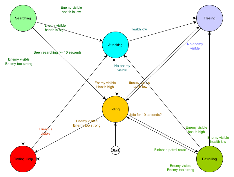
This captures the essence of the decision making for that agent based on the situation it finds itself in, with each arrow showing a transition between states, if the condition alongside the arrow is true.

Every update or ‘tick’ we check the agent’s current state, look through the list of transitions, and if the conditions are met for a transition, change to the new state. The Idling state will, every frame or tick, check whether the 10 second timer has expired, and if it has, trigger the transition to the Patrolling state. Similarly, the Attacking state will check if the agent’s health is low, and if so, transition to the Fleeing state.

That handles the transitions between states – but what about the behaviours associated with the states themselves? In terms of carrying out the actual behaviours for a given state, there are usually 2 types of ‘hook’ where we attach actions to the finite state machine:

Actions we take periodically, for example every frame or every ‘tick’, for the current state.
Actions we take when we transition from one state to another.

For an example of the first type, the Patrolling state will, every frame or tick, continue to move the agent along the patrol route. The Attacking state will, every frame or tick, attempt to launch an attack or move into a position where that is possible. And so on.

For the second type, consider the ‘If enemy visible and enemy is too strong → Finding Help’ transition. The agent must pick where to go to find help, and store that information so that the Finding Help state knows where to go. Similarly, within the Finding Help state, once help has been found the agent transitions back to the Attacking state, but at that point it will want to tell the friend about the threat, so there might be a “NotifyFriendOfThreat” action that occurs on that transition.

Again, we can see this system through the lense of Sense/Think/Act. The senses are embodied in the data used by the transition logic. The thinking is embodied by the transitions available in each state. And the acting is carried out by the actions taken periodically within a state or on the transitions between states.

This basic system works well, although some times the continual polling for the transition conditions can be expensive. For example, if every agent has to do complex calculations every frame to determine whether it can see any enemies in order to decide whether to transition from Patrolling to Attacking, that might waste a lot of CPU time. As we saw earlier, we can think of important changes in the world state as ‘events’ which can be processed as they happen. So instead of the state machine explicitly checking a “can my agent see the player?” transition condition every frame, you might have a separate visibility system perform these checks a little less frequently (e.g. 5 times a second), and emit a “Player Seen” event when the check passes. This gets given to the state machine which would now have a “Player Seen event received” transition condition and would respond to the event accordingly. The end behaviour is identical, except for the almost unnoticeable (and yet more realistic) delay in responding, but the performance is better, as a result of moving the Sense part of the system to a separate part of the program.

Hierarchical State Machines

This is all well and good, but large state machines can get awkward to work with. If we wanted to broaden the Attacking state by replacing it with separate MeleeAttacking and RangedAttacking states, we would have to alter the in-bound transitions in every state, now and in future, that needs to be able to transition to an Attacking state.

You probably also noticed that there are a lot of duplicated transitions in our example. Most of the transitions in the Idling state are identical to the ones in the Patrolling state, and it would be good to not have to duplicate that work, especially if we add more states similar to that. It might make sense to group Idling and Patrolling under some sort of shared label of ‘Non-Combat’ where there is just one shared set of transitions to combat states. If we represent this as a state in itself, we could consider Idling and Patrolling as ‘sub-states’ of that, which allows us to represent the whole system more effectively. Example, using a separate transition table for the new Non-Combat sub-state:

Main states:

State

Transition Condition

New State

Non-Combat

enemy visible and enemy is too strong

Finding Help

enemy visible and health high

Attacking

enemy visible and health low

Fleeing

Attacking

no enemy visible

Non-Combat

health low

Fleeing

no enemy visible

Non-Combat

Searching

have been searching for 10 seconds

Non-Combat

enemy visible and enemy is too strong

Finding Help

enemy visible and health high

Attacking

enemy visible and health low

Fleeing

Finding Help

friend visible

Attacking

Start state: Non-Combat

Non-Combat state:

State

Transition Condition

New State

Idling

have been idle for 10 seconds

Patrolling

finished patrol route

Idling

Start state: Idling

And in diagram form:

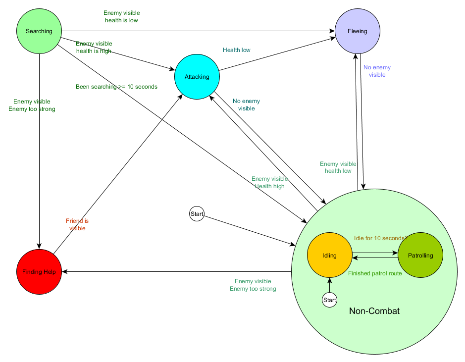
This is essentially the same system, except now there is a Non-Combat state which replaces Patrolling and Idling, and it is a state machine in itself, with 2 sub-states of Patrolling and Idling. With each state potentially containing a state machine of sub-states (and those sub-states perhaps containing their own state machine, for as far down as you need to go), we have a Hierarchical Finite State Machine (HFSM for short). By grouping the non-combat behaviours we cut out a bunch of redundant transitions, and we could do the same for any new states we chose to add that might share transitions. For example, if we expanded the Attacking state into MeleeAttacking and MissileAttacking states in future, they could be substates, transitioning between each other based on distance to enemy and ammunition availability, but sharing the exit transitions based on health levels and so on. Complex behaviours and sub-behaviours can be easily represented this way with a minimum of duplicated transitions.

Behavior Trees

With HFSMs we get the ability to build relatively complex behaviour sets in a relatively intuitive manner. However, one slight wrinkle in the design is that the decision making, in the form of the transition rules, is tightly-bound to the current state. In many games, that is exactly what you want. And careful use of a hierarchy of states can reduce the amount of transition duplication here. But sometimes you want rules that apply no matter which state you’re in, or which apply in almost all states. For example, if an agent’s health is down to 25%, you might want it to flee no matter whether it was currently in combat, or standing idle, or talking, or any other state, and you don’t want to have to remember to add that condition to every state you might ever add to a character in future. And if your designer later says that they want to change the threshold from 25% to 10%, you would then have to go through every single state’s relevant transition and change it.

Ideally for this situation you’d like a system where the decisions about which state to be in live outside the states themselves, so that you can make the change in just one place and still have it able to transition correctly. This is where a behaviour tree comes in.

There are several different ways to implement behaviour trees, but the essence is the same across most of them, and closely resembles the decision tree mentioned earlier: the algorithm starts at a ‘root node’ and there are nodes in the tree to represent either decisions or an action. However, there are a few key differences:

Nodes now return one of 3 values: Succeeded (if its work is done), Failed (if it cannot run), or Running (if it is still running and has not fully succeeded or failed yet).
We no longer have decision nodes to choose between 2 alternatives, but instead have ‘Decorator’ nodes, which have a single child node. If they ‘succeed’, they execute their single child node. Decorator nodes often have conditions in them which decides whether they succeed (and execute their subtree) or fail (and do nothing). They can also return Running if appropriate.
Nodes that take actions will return the Running value to represent activities that are ongoing

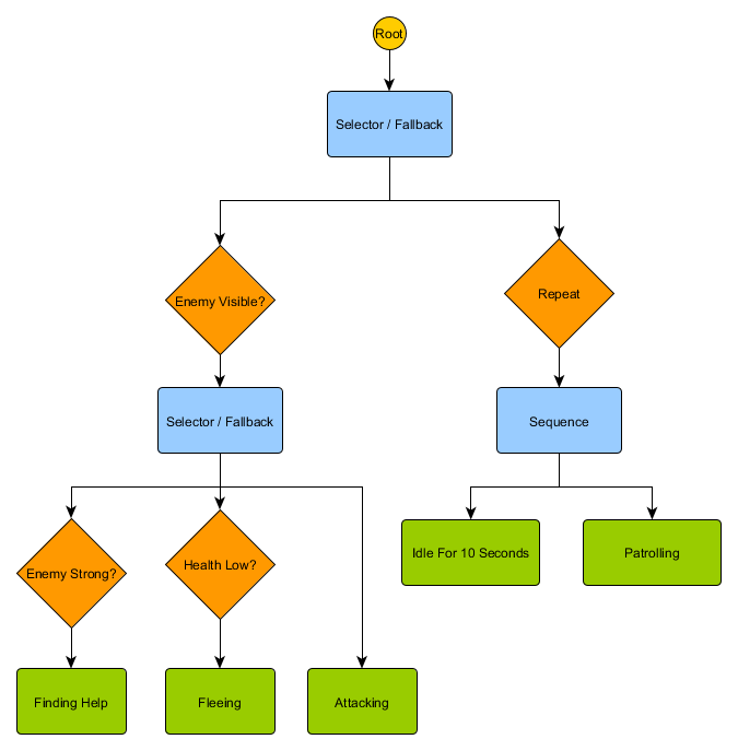
This small set of nodes can be combined to produce a large number of complex behaviours, and is often a very concise representation. For example, we can rewrite the guard’s hierarchical state machine from the previous example as a behaviour tree:

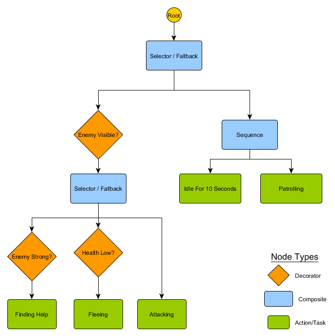
With this structure, there doesn’t need to be an explicit transition from the Idling or Patrolling states to the Attacking states or any others – if the tree is traversed top-down, left-to-right, the correct decision gets made based on the current situation. If an enemy is visible and the character’s health is low, the tree will stop execution at the ‘Fleeing’ node, regardless of what node it was previously executing - Patrolling, Idling, Attacking, etc.

You might notice that there’s currently no transition to return to Idling from the Patrolling state – this is where non-conditional decorators come in. A common decorator node is Repeat – this has no condition, but simply intercepts a child node returning ‘Succeeded’ and runs that child node again, returning ‘Running’ instead. The new tree looks like this:

Behaviour trees are quite complex as there are often many different ways to draw up the tree and finding the right combination of decorator and composite nodes can be tricky. There are also the issues of how often to check the tree (do we want traverse it every frame, or only when something happens that mean one of the conditions has changed?) and how to store state relating to the nodes (how do we know when we’ve been idling for 10 seconds? How do we know which nodes were executing last time, so we can handle a sequence correctly?) For this reason there are many different implementations. For example, some systems like the Unreal Engine 4 behaviour tree system have replaced decorator nodes with inline decorators, only re-evaluate the tree when the decorator conditions change, and provide ‘services’ to attach to nodes and provide periodic updates even when the tree isn’t being re-evaluated. Behaviour trees are powerful tools but learning to use them effectively, especially in the face of multiple varying implementations, can be daunting.

Utility-based systems

Some games would like to have a lot of different actions available, and therefore want the benefits of simpler, centralised transition rules, but perhaps don’t need the expressive power of a full behaviour tree implementation. Instead of having an explicit set of choices to make in turn, or a tree of potential actions with implicit fallback positions set by the tree structure, perhaps it’s possible to simply examine all the actions and pick out the one that seems most appropriate right now?

A utility-based system is exactly that – a system where an agent has a variety of actions at their disposal, and they choose one to execute based on the relative utility of each action, where utility is an arbitrary measure of how important or desirable performing that action is to the agent. By writing utility functions to calculate the utility for an action based on the current state of the agent and its environment, the agent is able to check those utility values and thereby select the most relevant state at any time.

Again, this closely resembles a finite state machine except one where the transitions are determined by the score for each potential state, including the current one. Note that we generally choose the highest-scoring action to transition to (or remain in, if already performing that action), but for more variety it could be a weighted random selection (favouring the highest scoring action but allowing some others to be chosen), picking a random action from the top 5 (or any other quantity), etc.

The typical utility system will assign some arbitrary range of utility values – say, 0 (completely undesirable) to 100 (completely desirable) and each action might have a set of considerations that influence how that value is calculated. Returning to our guard example, we might imagine something like this:

Action

Utility Calculation

FindingHelp

If enemy visible and enemy is strong and health low return 100 else return 0

Fleeing

If enemy visible and health low return 90 else return 0

Attacking

If enemy visible return 80

Idling

If currently idling and have done it for 10 seconds already, return 0, else return 50

Patrolling

If at end of patrol route, return 0, else return 50

One of the most important things to notice about this setup is that transitions between actions are completely implicit – any state can legally follow any other state. Also, action priorities are implicit in the utility values returned. If the enemy is visible and that enemy is strong and the character’s health is low then both Fleeing and FindingHelp will return high non-zero values, but FindingHelp always scores higher. Similarly, the non-combat actions never return more than 50, so they will always be trumped by a combat action. Actions and their utility calculiations need designing with this in mind.

Our example has actions return either a fixed constant utility value, or one of two fixed utility values. A more realistic system will typically involve returning a score from a continuous range of values. For example, the Fleeing action might return higher utility values if the agent’s health is lower, and the Attacking action might return lower utility values if the foe is too tough to beat. This would allow the Fleeing action to take precedence over Attacking in any situation where the agent feels that it doesn’t have enough health to take on the opponent. This allows relative action priorities to change based on any number of criteria, which can make this type of approach more flexible than a behavior tree or finite state machine.

Each action usually has a bunch of conditions involved in calculating the utility. To avoid hard-coding everything, this may need to be written in a scripting language, or as a series of mathematical formulae aggregated together in an understandable way. See Dave Mark’s (@IADaveMark) lectures and presentations for a lot more information about this.

Some games that attempt to model a character’s daily routine, like The Sims, add an extra layer of calculation where the agent has a set of ‘drives’ or ‘motivations’ that influence the utility scores. For example, if a character has a Hunger motivation, this might periodically go up over time, and the utility score for the EatFood action will return higher and higher values as time goes on, until the character is able to execute that action, decrease their Hunger level, and the EatFood action then goes back to returning a zero or near-zero utility value.

The idea of choosing actions based on a scoring system is quite straightforward, so it is obviously possible – and common – to use utility-based decision making as a part of other AI decision-making processes, rather than as a full replacement for them. A decision tree could query the utility score of its two child nodes and pick the higher-scoring one. Similarly a behaviour tree could have a Utility composite node that uses utility scores to decide which child to execute.

Movement and Navigation

In our previous examples, we either had a simple paddle which we told to move left or right, or a guard character who was told to patrol or attack. But how exactly do we handle movement of an agent over a period of time? How do we set the speed, how do we avoid obstacles, and how do we plan a route when getting to the destination is more complex than moving directly? We’ll take a look at this now.

Steering

At a very basic level, it often makes sense to treat each agent as having a velocity value, which encompasses both how fast it is moving and in which direction. This velocity might be measured in metres per second, miles per hour, pixels per second, etc. Recalling our Sense/Think/Act cycle, we can imagine that the Think part might choose a velocity, and then the Act part applies that velocity to the agent, moving it through the world. It’s common for games to have a physics system that performs this task for you, examining the velocity value of every entity and adjusting the position accordingly, so you can often delegate this work to that system, leaving the AI just with the job of deciding what velocity the agent should have.

If we know where an agent wishes to be, then we will want to use our velocity to move the agent in that direction. Very trivially, we have an equation like this:


desired_travel = destination_position – agent_position

So, imagining a 2D world where the agent is at (-2,-2) and the destination is somewhere roughly to the north-east at (30, 20) the desired travel for the agent to get there is (32, 22). Let’s pretend these positions are in metres - if we decide that our agent can move 5 metres per second then we would scale our travel vector down to that size and see that we want to set a velocity of roughly (4.12, 2.83). With that set, and movement being based on that value, the agent would arrive at the destination a little under 8 seconds later, as we would expect.

The calculations can be re-run whenever you want. For example, if the agent above was half-way to the target, the desired travel would be half the length, but once scaled to the agent’s maximum speed of 5 m/s the velocity comes out the same. This also works for moving targets (within reason), allowing the agent to make small corrections as they move.

Often we want a bit more control than this – for example, we might want to ramp up the velocity slowly at the start to represent a person moving from a stand still, through to walking, and then to running. We might want to do the same at the other end to have them slow down to a stop as they approach the destination. This is often handled by what are known as “steering behaviours”, each with specific names like Seek, Flee, Arrival, and so on. The idea of these is that acceleration forces can be applied to the agent’s velocity, based on comparing the agent’s position and current velocity to the destination position, to produce different ways to move towards a target.

Each behaviour has a slightly different purpose. Seek and Arrive are ways of moving an agent towards a destination point. Obstacle Avoidance and Separation help an agent take small corrective movements to steer around small obstacles between the agent and its destination. Alignment and Cohesion keep agents moving together to simulate flocking animals. Any number of these different steering behaviours can be added together, often as a weighted sum, to produce an aggregate value that takes these different concerns into account and produces a single output vector. For example, you might see a typical character agent use an Arrival steering behaviour alongside a Separation behaviour and an Obstacle Avoidance behaviour to keep away from walls and other agents. This approach works well in fairly open environments that aren’t too complex or crowded.

However, in more challenging environments, simply adding together the outputs from the behaviours doesn’t work well – perhaps they result in moving too slowly past an object, or an agent gets stuck when the Arrival behaviour wants to go through an obstacle but the Obstacle Avoidance behaviour is pushing the agent back the way it came. Therefore it sometimes makes sense to consider variations on steering behaviours which are more sophisticated than just adding together all the values. One family of approaches is to think of steering the other way around – instead of having each of the behaviours give us a direction and then combine them to reach a consensus (which may itself not be adequate), we could instead consider steering in several different directions - such as 8 compass points, or 5 or 6 directions in front of the agent - and see which one of those is best.

Still, in a complex environment with dead-ends and choices over which way to turn, we’re going to need something more advanced, which we’ll come to shortly.

Pathfinding

That’s great for simple movement in a fairly open area, like a soccer pitch or an arena, where getting from A to B is mostly about travelling in a straight line with small corrections to avoid obstacles. But what about when the route to the destination is more complex? This is where we need ‘pathfinding’, which is the act of examining the world and deciding on a route through it to get the agent to the destination.

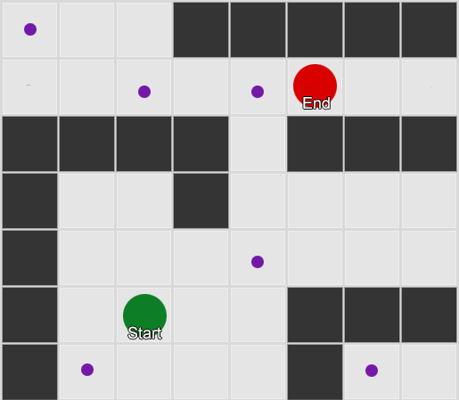
Simplest – overlay a grid, for each square near to you, look at the neighbors you’re allowed to move into. If any of those are the destination, follow the route back from each square to the previous until you get to the start, and that’s the route. Otherwise, repeat the process with the reachable neighbors of the previous neighbors, until you find the destination or run out of squares (which means there is no possible route). This is what is formally known as a Breadth-First Search algorithm (often abbreviated to BFS) because at each step it looks at all directions (hence ‘breadth’) before moving the search outwards. The search space is like a wavefront that moves out until it hits the place that is being searched for.

This is a simple example of the search in action. The search area expands at each step until it has included the destination point – then the path back to the start can be traced.

The result here is that you get a list of gridsquares which make up the route you need to take. This is commonly called the ‘path’ (hence pathfinding) but you can also think of it as a plan as it represents a list of places to be, one after the other, to achieve the final goal of being at the destination.

Now, given that we will know the position of each gridsquare in the world, it’s possible to use the steering behaviours mentioned previously to move along the path – first from the start node to node 2, then from node 2 to node 3, and so on. The simplest approach is to steer towards the centre of the next gridsquare, but a popular alternative is to steer for the middle of the edge between the current square and the next one. This allows the agent to cut corners on sharp turns which can make for more realistic-looking movement.

It’s easy to see that this algorithm can be a bit wasteful, as it explores just as many squares in the ‘wrong’ direction as the ‘right’ direction. It also doesn’t make any allowances for movement costs, where some squares are more expensive than others. This is where a more sophisticated algorithm called A* (pronounced ‘A star’) comes in. It works much the same way as breadth-first search, except that instead of blindly exploring neighbors, then neighbors of neighbors, then neighbors of neighbors of neighbors and so on, it puts all these nodes into a list and sorts them so that the next node it explores is always the one it thinks is most likely to lead to the shortest route. The nodes are sorted based on a heuristic – basically an educated guess – that takes into account 2 things – the cost of the hypothetical route to that gridsquare (thus incorporating any movement costs you need) and an estimate of how far that gridsquare is from the destination (thus biasing the search in the right direction).

In this example we show it examining one square at a time, each time picking a neighbouring square that is the best (or joint best) prospect. The resulting path is the same as with breadth-first search, but fewer squares were examined in the process – and this makes a big difference to the game's performance on complex levels.

Movement without a grid

The previous examples used a grid overlaid on the world and plotted a route across the world in terms of the gridsquares. But most games are not laid out on a grid, and overlaying a grid might therefore not make for realistic movement patterns. It might also require compromises over how large or small to make each gridsquare – too large, and it doesn’t adequately represent small corridors or turnings, too small and there could be thousands of gridsquares to search which will take too long. So, what are the alternatives?

The first thing to realise is that, in mathematical terms, the grid gives us a ‘graph’ of connected nodes. The A* (and BFS) algorithms actually operate on graphs, and don’t care about our grid at all. So we could decide to place the nodes at arbitrary positions in the world, and providing there is a walkable straight line between any two connected nodes, and between the start and end positions and at least one of the nodes, our algorithm will work just as well as before – usually better, in fact, because we have fewer nodes to search. This is often called a ‘waypoints’ system as each node represents a significant position in the world that can form part of any number of hypothetical paths.

Example 1: a node in every grid square. The search starts from the node the agent is in, and ends at the node in the target gridsquare.

Example 2: a much smaller set of nodes, or waypoints. The search begins at the agent, passes through as many waypoints as necessary, and then proceeds to the end point. Note that moving to the first waypoint, south-west of the player, is an inefficient route, so some degree of post-processing of a path generated in this way is usually necessary (for example, to spot that the path can go directly to the waypoint to the north-east).

This is quite a flexible and powerful system. But it usually requires some care in deciding where and how to place the waypoints, otherwise agents might not be able to see their nearest waypoint and start a path. It would be great if we could generate the waypoints automatically based on the world geometry somehow.

This is where a ‘navmesh’ comes in. Short for ‘navigation mesh’ it is a (typically) 2D mesh of triangles that roughly overlays the world geometry, anywhere that the game allows an agent to walk. Each of the triangles in the mesh becomes a node in the graph and has up to 3 adjacent triangles which become neighboring nodes in the graph.

This picture is an example from the Unity engine – it has analysed the geometry in the world and produced a navmesh (light blue) that is an approximation of it. Each polygon in the navmesh is an area that an agent can stand on, and the agent is able to move from one polygon to any polygon adjacent to it. (In this example the polygons are narrower than the floors they rest upon, to take account of the agent’s radius that would extend out beyond the agent’s nominal position.)

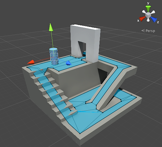
We can search for a route through this mesh, again using A*, and this gives us a near-perfect route through the world that can take all the geometry into account and yet not require an excess of redundant nodes (like the grid) or require a human to generate waypoints.

Pathfinding is a wide subject and there are many different approaches to it, especially if you have to code the low level details yourself. One of the best sources for further reading is Amit Patel’s site.

Planning

We saw with pathfinding that sometimes it’s not sufficient to just pick a direction and move straight there – we have to pick a route and make several turns in order to reach the destination that we want. We can generalise this idea to a wide range of concepts where achieving your goal is not just about the next step, but about a series of steps that are necessary to get there, and where you might need to look ahead several steps in order to know what the first one should be. This is what we call planning. Pathfinding can be thought of as one specific application of planning, but there are many more applications for the concept. In terms of our Sense/Think/Act cycle, this is where the Think phase tries to plan out multiple Act phases for the future.

Let’s look at the game Magic: The Gathering. It’s your first turn, you have a hand of cards, and the hand includes a Swamp which provides 1 point of Black Mana, a Forest which provides 1 point of Green Mana, a Fugitive Wizard which requires 1 Blue Mana to summon, and an Elvish Mystic which requires 1 Green Mana to summon. (We’ll ignore the other 3 cards for now to keep this simple.) The rules say (roughly) that a player is allowed to play 1 land card per turn, can ‘tap’ their land cards in play to extract the mana from it, and can cast as many spells (including creature summoning) as they have available mana. In this situation a human player would probably know to play the Forest, tap it for 1 point of Green Mana, and then summon the Elvish Mystic. But how would a game AI know to make that decision?

A Simple ‘Planner’

The naive approach might be to just keep trying each action in turn until no appropriate ones are left. Looking at the hand of cards, it might see that it can play the Swamp, so it does so. After that, does it have any other actions left this turn? It can’t summon either the Elvish Mystic or the Fugitive Wizard as they require green and blue mana respectively, and our Swamp in play can only provide black mana. And we can’t play the Forest because we’ve already played the Swamp. So, the AI player has produced a valid turn, but not a very optimal one. Luckily, we can do better.

In much the same way that pathfinding finds a list of positions to move through the world to reach a desired position, our planner can find a list of actions that get the game into a desired state. Just like each position along a path had a set of neighbors which were potential choices for the next step along the path, each action in a plan has neighbors, or ‘successors’, which are candidates for the next step in the plan. We can search through these actions and successor actions until we reach the state that we want.

In our example, let’s assume the desired outcome is “to summon a creature, if possible”. The start of the turn sees us with only 2 potential actions allowed by the rules of the game:


1. Play the Swamp (result: Swamp leaves the Hand, enters play)
2. Play the Forest (result: Forest leaves the Hand, enters play)

Each action taken may enable further actions and close off others, again depending on the game rules. Imagine we choose to play the swamp – this removes that action as a potential successor (as the swamp has already been played), it removes Play The Forest as a successor (because the game rules only allow you to play one Land card per turn), and it adds Tap the Swamp for 1 point of Black Mana as a successor – the only successor, in fact. If we follow it one step further and choose ‘Tap The Swamp’, we get 1 point of black mana that we can’t do anything with, which is pointless.


1. Play the Swamp (result: Swamp leaves the Hand, enters play)
            1.1 Tap the Swamp (result: Swamp is tapped, +1 Black mana available)
                        No actions left – END
2. Play the Forest (result: Forest leaves the Hand, enters play)

This short list of actions didn’t achieve much, leading us down the equivalent of a dead-end if we use the pathfinding analogy. So, we repeat the process for the next action. We choose ‘Play The Forest’ - again, this removes ‘Play The Forest’ and ‘Play The Swamp’ from consideration, and opens up ‘Tap The Forest’ as the potential (and only) next step. That gives us 1 green mana, which in this case opens up a third step, that of Summon Elvish Mystic.


1. Play the Swamp (result: Swamp leaves the Hand, enters play)
           1.1. Tap the Swamp (result: Swamp is tapped, +1 Black mana available)
                       No actions left – END
2. Play the Forest (result: Forest leaves the Hand, enters play)
            2.1 Tap the Forest  (result: Forest is tapped, +1 Green mana available)
                        2.1.1 Summon Elvish Mystic (result: Elvish Mystic in play, -1 Green mana available)
                                    No actions left – END

We’ve now explored all the possible actions, and the actions that follow on from those actions, and we found a plan that allowed us to summon a creature: Play the Forest, Tap the Forest, Summon the Elvish Mystic.

Obviously this is a very simplified example, and usually you would want to pick the best plan rather than just any plan that meets some sort of criteria (such as ‘summon a creature’). Typically you might score potential plans based on the final outcome or the cumulative benefit of following the plan. For example, you might award yourself 1 point for playing a Land card and 3 points for summoning a creature. “Play The Swamp” would be a short plan yielding 1 point, but “Play The Forest → Tap The Forest → Summon Elvish Mystic” is a plan yielding 4 points, 1 for the land and 3 for the creature. This would be the top scoring plan on offer and therefore would be chosen, if that was how we were scoring them.

We’ve shown how planning works within a single turn of Magic: The Gathering, but it can apply just as well to actions in consecutive turns (e.g. moving a pawn to make room to develop a bishop in Chess, or dashing to cover in XCOM so that the unit can shoot from safety next turn) or to an overall strategy over time (e.g. choosing to construct pylons before other Protoss buildings in Starcraft, or quaffing a Fortify Health potion in Skyrim before attacking an enemy).

Improved Planning

Sometimes there are just too many possible actions at each step for it to be reasonable for us to consider every permutation. Returning to the Magic: The Gathering example - imagine if we had several creatures in our hand, plenty of land already in play so we could summon any of them, creatures already in play with some abilities available, and a couple more land cards in our hand – the number of permutations of playing lands, tapping lands, summoning creatures, and using creature abilities, could number in the thousands or even tens of thousands. Luckily we have a couple of ways to attempt to manage this.

The first way is ‘backwards chaining’. Instead of trying all the actions and seeing where they lead, we might start with each of the final results that we want and see if we can find a direct route there. An analogy is trying to reach a specific leaf from the trunk of a tree – it makes more sense to start from that leaf and work backwards, tracing the route easily to the trunk (which we could then follow in reverse), rather than starting from the trunk and trying to guess which branch to take at each step. By starting at the end and going in reverse, forming the plan can be a lot quicker and easier.

For example, if the opponent is on 1 health point, it might be useful to try and find a plan for “Deal 1 or more points of direct damage to the opponent”. To achieve this, our system knows it needs to cast a direct damage spell, which in turn means that it needs to have one in the hand and have enough mana to cast it, which in turn means it must be able to tap sufficient land to get that mana, which might require it to play an additional land card.

Another way is ‘best-first search’. Instead of iterating through all permutations of action exhaustively, we measure how ‘good’ each partial plan is (similarly to how we chose between plans above) and we evaluate the best-looking one each time. This often allows us to form a plan that is optimal, or at least good enough, without needing to consider every possible permutation of plans. A* is a form of best-first search – by exploring the most promising routes first it can usually find a path to the destination without needing to explore too far in other directions.

An interesting and increasingly popular variant on best-first search is Monte Carlo Tree Search. Instead of attempting to guess which plans are better than others while selecting each successive action, it picks random successors at each step until it reaches the end when no more actions are available – perhaps because the hypothetical plan led to a win or lose condition – and uses that outcome to weight the previous choices higher or lower. By repeating this process many times in succession it can produce a good estimate of which next step is best, even if the situation changes (such as the opponent taking preventative action to thwart us).

Finally, no discussion of planning in games is complete without mentioning Goal-Oriented Action Planning, or GOAP for short. This is a widely-used and widely-discussed technique, but apart from a few specific implementation details it is essentially a backwards-chaining planner that starts with a goal and attempts to pick an action that will meet that goal, or, more likely, a list of actions that will lead to the goal being met. For example, if the goal was e.g. “Kill The Player”, and the player is in cover, the plan might be “FlushOutWithGrenade”→ “Draw Weapon” → “Attack”.

There are typically several goals, each with their own priority, and if the highest priority goal can’t be met – e.g. no set of actions can form a “Kill the player” plan because the player is not visible – it will fall back to lower priority goals, such as “Patrol” or “Stand guard”.

Learning and Adapting

We mentioned at the start that game AI does not generally use ‘machine learning’ because it is not generally suited to real-time control of intelligent agents in a game world. However, that doesn’t mean we can’t take some inspiration from that area when it makes sense. We might want a computer opponent in a shooter game to learn the best places to go in order to score the most kills. Or we might want the opponent in a fighting game like Tekken or Street Fighter to spot when we use the same ‘combo’ move over and over and start blocking it, forcing us to try different tactics. So there are times when some degree of machine learning can be useful.

Statistics and Probabilities

Before we look at more complex examples, it’s worth considering how far we can go just by taking some simple measurements and using that data to make decisions. For example, say we had a real-time strategy game and we were trying to guess whether a player is likely to launch a rush attack in the first few minutes or not, so we can decide whether we need to build more defences or not. We might want to extrapolate from the player’s past behaviour to give an indication of what the future behaviour might be like. To begin with we have no data about the player from which to extrapolate – but each time the AI plays against the human opponent, it can record the time of the first attack. After several plays, those times can be averaged and will be a reasonably good approximation of when that player might attack in future.

The problem with simple averages is that they tend towards the centre over time, so if a player employed a rushing strategy the first 20 times and switched to a much slower strategy the next 20 times, the average would be somewhere in the middle, telling us nothing useful. One way to rectify this is a simple windowed average, such as only considering the last 20 data points.

A similar approach can be used when estimating the probability of certain actions happening, by assuming that past player preferences will carry forward to the future. For example, if a player attacks us with a Fireball 5 times, a Lightning Bolt 2 times, and hand-to-hand combat just once, it’s likely that they prefer the Fireball, using 5 in 8 times. Extrapolating from this, we can see the probability of different weapon use is Fireball=62.5%, Lightning Bolt=25%, and Hand-To-Hand=12.5%. Our AI characters would be well advised to find some fire-retardant armor!

Another interesting method is to use a Naive Bayes Classifier to examine large amounts of input data and try to classify the current situation so the AI agent can react appropriately. Bayesian classifiers are perhaps best known for their use in email spam filters, where they examine the words in the email, compare them to whether those words mostly appeared in spam or non-spam in the past, and use that to make a judgement on whether this latest email is likely to be spam. We could do similarly, albeit with less input data. By recording all the useful information we see (such as which enemy units are constructed, or which spells they use, or which technologies they have researched) and then noting the resulting situation (war vs peace, rush strategy vs defensive strategy, etc.), we could pick appropriate behaviour based on that.

With all of these learning approaches, it might be sufficient – and often preferable – to run them on the data gathered during playtesting prior to release. This allows the AI to adapt to the different strategies that your playtesters use, but won’t change after release. By comparison, AI that adapts to the player after release might end up becoming too predictable or even too difficult to beat.

Basic weight-based adaptation

Let’s take things a little further. Rather than just using the input data to choose between discrete pre-programmed strategies, maybe we want to change a set of values that inform our decision making. Given a good understanding of our game world and game rules, we can do the following:

Have the AI collect data about the state of the world and key events during play (as above);
Change several values or ‘weights’ based on that data as it is being collected;
Implement our decisions based on processing or evaluating these weights.

Imagine the computer agent has several major rooms in a FPS map to choose from. Each room has a weight which determines how desirable that room is to visit, all starting at the same value. When choosing where to go, it picks a room at random, but biased based on those weights. Now imagine that when the computer agent is killed, it notes which room it was in and decreases the weight, so it is less likely to come back here in future. Similarly, imagine the computer agent scores a kill – it might increase the weight of the room it’s in, to move it up the list of preferences. So if one room starts being particularly deadly for the AI player, it’ll start to avoid it in future, but if some other room lets the AI score a lot of kills, it’ll keep going back there.

Markov Models

What if we wanted to use data collected like this to make predictions? For example, if we record each room we see a player in over a period of time as they play the game, we might reasonably expect to use that to predict which room the player might move to next. By keeping track of both the current room the player is in and the previous room they were seen in, and recording that as a pair of values, we can calculate how often each of the former situations leads to the latter situation and use that for future predictions.

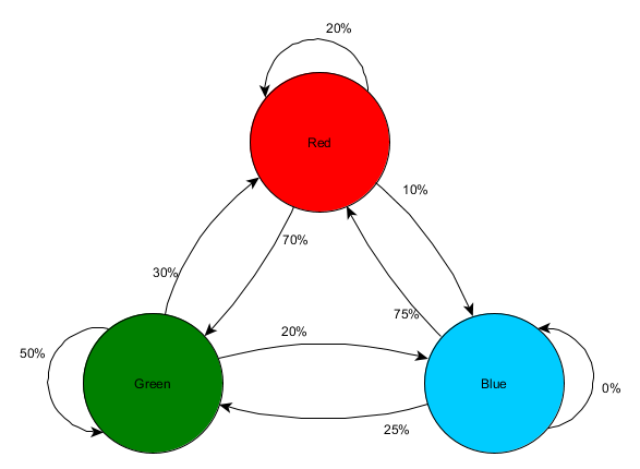
Imagine there are 3 rooms, Red, Green, and Blue, and these are the observations we saw when watching a play session:

First Room Seen

Total Observations

Next Room Seen

Times Observed

Percentage

Red

20%

Green

70%

Blue

10%

Green

Red

30%

Green

50%

Blue

20%

Blue

Red

75%

Green

25%

Blue

The number of sightings in each room is fairly even, so it doesn’t tell us much about where might be a good place to place an ambush. It might be skewed by players spawning evenly across the map, equally likely to emerge into any of those three rooms. But the data about the next room they enter might be useful, and could help us predict a player’s movement through the map.

We can see at a glance that the Green room is apparently quite desirable to players – most people in the Red room then proceed to the Green room, and 50% of players seen in the Green room are still there the next time we check. We can also see that the Blue room is quite an undesirable destination – people rarely pass from the Red or Green rooms to the Blue room, and nobody seems to linger in the Blue room at all.

But the data tells us something more specific – it says that when a player is in the Blue room, the next room we see them in is most likely to be the Red room, not the Green room. Despite the Green room being a more popular destination overall than the Red one, that trend is slightly reversed if the player is currently in the Blue room. The next state (i.e. the room they choose to travel to) is apparently dependent on the previous state (i.e. the room they currently find themselves in) so this data lets us make better predictions about their behaviour than if we just counted the observations independently.

This idea that we can use knowledge of the past state to predict a future state is called a Markov model and examples like this where we have accurately measurable events (such as ‘what room is the player in’) are called Markov Chains. Since they represent the chance of changes between successive states they are often visually represented as a finite state machine with the probability shown alongside each transition. Previously we used a state machine to represent some sort of behavioural state that an agent was in, but the concept extends to any sort of state, whether to do with an agent or not. In this case the states represent the room the agent is occupying, and it would look like this:

This is a simple approach to represent the relative chance of different state transitions, giving the AI some predictive power regarding the next state. But we could go further, by using the system to look 2 or more steps into the future.

If the player is seen in the Green room, we use our data to estimate there is a 50% chance they will still be in the Green room for the next observation. But what’s the chance they will still be there for the observation after that? It’s not just the chance that they stayed in the Green room for 2 observations (50% * 50% = 25%) but also the chance that they left and came back. Here’s a new table with the previous values applied to 3 observations, 1 current and 2 hypothetical ones in the future.

Observation 1

Hypothetical Observation 2

Percentage chance

Hypothetical Observation 3

Percentage chance

Cumulative chance

Green

Red

30%

Red

20%

Green

70%

21%

Blue

10%

Green

50%

Red

30%

15%

Green

50%

25%

Blue

20%

10%

Blue

20%

Red

75%

15%

Green

25%

Blue

Total:

100%

Here we can see that the chance of seeing the player in the Green room 2 observations later is likely to be 51% - 21% of that coming from a journey via the Red room, 5% of it seeing the player visit the Blue room in between, and 25% staying in the Green room throughout.

The table is just a visual aid – the procedure requires only that you multiply out the probabilities at each step. This means you could look a long way into the future, with one significant caveat: we are making an assumption that the chance of entering a room depends entirely on the current room they are in. This is what we call the Markov Property – the idea that a future state depends only on the present state. While it allows us to use powerful tools like this Markov Chain, it is usually only an approximation. Players may change which room they are in based on other factors, such as their health level or how much ammo they have, and since we don’t capture this information as part of our state our predictions will be less accurate as a result.

N-Grams

What about our fighting game combo-spotting example? This is a similar situation, where we want to predict a future state based on the past state (in order to decide how to block or evade an attack), but rather than looking at a single state or event, we want to look for sequences of events that make up a combo move.

One way to do this is to store each input (such as Kick, Punch, or Block) in a buffer and record the whole buffer as the event. So, imagine a player repeatedly presses Kick, Kick, Punch to use a ‘SuperDeathFist’ attack, the AI system stores all the inputs in a buffer, and remembers the last 3 inputs used at each step.

Input

Input sequence so far

New input memory

Kick

none

Punch

Kick, Punch

none

Kick

Kick, Punch, Kick

Kick

Kick, Punch, Kick, Kick

Punch, Kick, Kick

Punch

Kick, Punch, Kick, Kick, Punch

Kick, Kick, Punch

Block

Kick, Punch, Kick, Kick, Punch, Block

Kick, Punch, Block

Kick

Kick, Punch, Kick, Kick, Punch, Block, Kick

Punch, Block, Kick

Kick

Kick, Punch, Kick, Kick, Punch, Block, Kick, Kick

Block, Kick, Kick

Punch

Kick, Punch, Kick, Kick, Punch, Block, Kick, Kick, Punch

Kick, Kick, Punch

(Rows in bold are when the player launches the SuperDeathFist attack.)

It would be possible to look at all the times that the player chose Kick followed by another Kick in the past, and then notice that the next input is always Punch. This lets the AI agent make a prediction that if the player has just chosen Kick followed by Kick, they are likely to choose Punch next, thereby triggering the SuperDeathFist. This allows the AI to consider picking an action that counteracts that, such as a block or evasive action.

These sequences of events are known as N-grams where N is the number of items stored. In the previous example it was a 3-gram, also known as a trigram, which means the first 2 entries are used to predict the 3rd one. In a 5-gram, the first 4 entries would hopefully predict the 5th, and so on.

The developer needs to choose the size (sometimes called the ‘order’) of the N-grams carefully. Lower numbers require less memory, as there are fewer possible permutations, but they store less history and therefore lose context. For instance, a 2-gram (sometimes called a ‘bigram’) would have entries for Kick, Kick and entries for Kick, Punch but has no way of storing Kick, Kick, Punch, so has no specific awareness of that combo.

On the other hand, higher numbers require more memory and are likely to be harder to train, as you will have many more possible permutations and therefore you might never see the same one twice. For example, if you had the 3 possible inputs of Kick, Punch, or Block and were using 10-grams then you have almost 60,000 different permutations.

A bigram model is basically a trivial Markov Chain – each ‘Past State/Current State’ pair is a bi-gram and you can predict the second state based on the first. Tri-grams and larger N-grams can also be thought of as Markov Chains, where all but the last item in the N-gram together form the first state and the last item is the second state. Our fighting game example is representing the chance of moving from the Kick then Kick state to the Kick then Punch state. By treating multiple entries of input history as a single unit, we are essentially transforming the input sequence into one piece of state, which gives us the Markov Property – allowing us to use Markov Chains to predict the next input, and thus to guess which combo move is coming next.

Knowledge representation

We’ve discussed several ways of making decisions, making plans, and making predictions, and all of these are based on the agent’s observations of the state of the world. But how do we observe a whole game world effectively? We saw earlier that the way we represent the geography of the world can have a big effect on how we navigate it, so it is easy to imagine that this holds true about other aspects of game AI as well. How do we gather and organise all the information we need in a way that performs well (so it can be updated often and used by many agents) and is practical (so that the information is easy to use with our decision-making)? How do we turn mere data into information or knowledge? This will vary from game to game, but there are a few common approaches that are widely used.

Smart Objects

Tags are a way of putting extra information into the agent’s environment to help it understand the options available to it, so that queries like “Find me every place nearby that provides cover” or “Find me every enemy in range that is a spellcaster” can be executed efficiently and will work on future game assets with minimal effort required. But sometimes tags don’t contain enough information to be as useful as we need.

Imagine a medieval city simulator, where the adventurers within wander around of their own accord, training, fighting, and resting as necessary. We could place training grounds around the city, and give them a ‘TRAINING’ tag, so that it’s easy for the adventurers to find where to train. But let’s imagine one is an archery range, and the other is a school for wizards – we’d want to show different animations in each case, because they represent quite different activities under the generic banner of ‘training’, and not every adventurer will be interested in both. We might decide to drill down and have ARCHERY-TRAINING and MAGIC-TRAINING tags, and separate training routines for each one, with the specific animations built in to those routines. That works. But imagine your design team then say, “Let’s have a Robin Hood Training School, which offers archery and swordfighting”! And now swordfighting is in, they then ask for “Gandalf’s Academy of Spells and Swordfighting”. You find yourself needing to support multiple tags per location, looking up different animations based on which aspect of the training the adventurer needs, etc.

Another way would be to store this information directly in the object, along with the effect it has on the player, so that the AI can simply be told what the options are, and select from them accordingly based on the agent’s needs. It can then move to the relevant place, perform the relevant animation (or any other prerequisite activity) as specified by the object, and gain the rewards accordingly.

Animation to Perform

Result for User

Archery Range

Shoot-Arrow

+10 Archery Skill

Magic School

Sword-Duel

+10 Swords Skill

Robin Hood’s School

Shoot-Arrow

+15 Archery Skill

Sword-Duel

+8 Swords Skill

Gandalf’s Academy

Sword-Duel

+5 Swords Skill

Cast-Spell

+10 Magic Skill

An archer character in the vicinity of the above 4 locations would be given these 6 options, of which 4 are irrelevant as the character is neither a sword user nor a magic user. By matching on the outcome, in this case, the improvement in skill, rather than on a name or a tag, we make it easy to extend our world with new behaviour. We can add Inns for rest and food. We could allow adventurers to go to the Library and read about spells, but also about advanced archery techniques.

Object Name

Animation to Perform

End Result

Inn

Buy

-10 Hunger

Inn

Sleep

-50 Tiredness

Library

Read-Book

+10 Spellcasting Skill

Library

Read-Book

+5 Archery Skill

If we just had a “Train In Archery” behaviour, even if we tagged our Library as a ARCHERY-TRAINING location, we would presumably still need a special case to handle using the ‘read-book’ animation instead of the usual swordfighting animation. This system gives us more flexibility by moving these associations into data and storing the data in the world.

By having the objects or locations – like the Library, the Inn, or the training schools – tell us what services they offer, and what the character must do to obtain them, we get to use a small number of animations and simple descriptions of the outcome to enable a vast number of interesting behaviours. Instead of objects passively waiting to be queried, those objects can instead give out a lot of information about what they can be used for, and how to use them.

Response Curves

Often you have a situation where part of the world state can be measured as a continuous value – for example:

“Health Percentage” typically ranges from 0 (dead) to 100 (in perfect health)
“Distance To Nearest Enemy” ranges from 0 to some arbitrary positive value

You also might have some aspect of your AI system that requires continuous-valued inputs in some other range. For example, a utility system might want to take both the distance to the nearest enemy and the character’s current health when deciding whether to flee or not.

However, the system can’t just add the two world state values to create some sort of ‘safeness’ level because the two units are not comparable – it would consider a near-dead character almost 200 units from an enemy to be just as safe as a character in perfect health who was 100 units from an enemy. Similarly, while the health percentage value is broadly linear, the distance is not – the difference between an enemy being 200m away and 190m away is much less significant than the difference between an enemy 10m away and one right in front of the character.

Ideally, we want an approach that can take these 2 measurements and convert them into similar ranges so that they can be directly compared. And we want designers to be able to choose how these conversions work, so that they can control the relative importance of each value. Response Curves are a tool to do just that.

The simplest explanation of a response curve is that it’s a graph with input along the X axis, the arbitrary values like “distance to nearest enemy”, and output along the Y axis, usually a normalized value from 0.0 to 1.0. The line or curve through the graph determines the mapping from the input to the normalized output, and designers tweak those lines to get the behavior they want.

For our “safeness” level calculation, we might decide to keep the health percentage as a linear value – i.e. 10% more health is equally good whether we’re badly injured or lightly injured – so mapping it to the 0 to 1 range is straightforward:

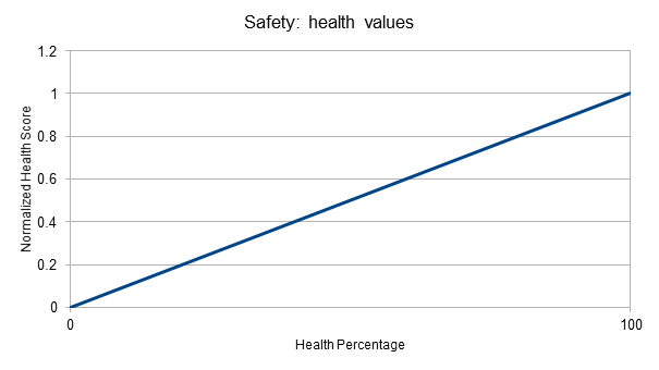
The distance to the nearest enemy is a bit different, since we presumably don’t care at all about enemies beyond a certain distance – let’s say 50 metres – and we care a lot more about the differences at close range than at long range.

Here we can see that the ‘safety’ output for an enemy at 40 or 50 metres is very similar: 0.96 vs 1.0.

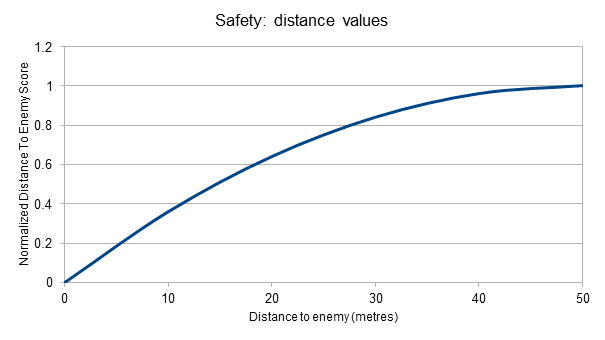
However, there’s a bigger safety difference between an enemy 15 metres away – roughly 0.5 – and an enemy 5 metres away – roughly 0.2. This better reflects the urgency that applies as an enemy draws nearer.

With these 2 values both scaled into the 0 to 1 range, we could calculate the overall Safety value as the average of the two input values. A character with 20% health and an enemy 50 metres away could have a Safety score of 0.6. A character with 75% health and an enemy just 5 metres away could have a Safety score of 0.47. And a badly wounded character with 10% health and an enemy just 5 metres away would have a Safety score of just 0.145.

Some things to bear in mind:

It’s common to use some sort of weighted average to combine the output of response curves into the final value – this makes it easier to re-use the same curves for calculating different values, by using different weights in each case to reflect the differing importance.
When the input value is outside the prescribed range – for example, an enemy more than 50m away in our example above – it’s common to clamp the input value to the maximum so the calculation acts as if they were at that range.
Implementation of the response curve will often take the form of a mathematical equation, typically running the (perhaps clamped) input through a linear equation or simple polynomial. But any system that allows a designer to create and evaluate a curve may suffice – for example, the Unity AnimationCurve object allows for the placement of arbitrary values, the choice of whether to smooth the line between the values or not, and the evaluation of any point along the line.

Blackboards

Often we find ourselves in a situation where the AI for an agent needs to start keeping track of knowledge and information it is picking up during play so that it can be used in future decision making. Maybe an agent needs to remember who the last character to attack it was, so that it knows that should be the focus of attacks in the short term. Or maybe it wants to note how long it was since it heard a disturbance, so that after some period of time it can stop investigating and go back to whatever it was doing before. Often the system that writes the data is quite separate from the system that reads the data, so it needs to be easily accessible from the agent rather than built in to the various AI systems directly. The reads may happen some time after the writes, so it needs to be stored somewhere that it can be retrieved later (rather than being calculated on demand, which may not be possible).

In a hard-coded AI system the answer here is usually just to add the necessary variables as the need for them arises. These variables go into the character or agent instances, either directly inline, or in the form of a separate structure or class to hold this information. AI routines are adapted to read and write from this data as needed. This works well as a simple approach, but can get unwieldy as more and more pieces of information need adding, and usually requires rebuilding the game each time.

A more advanced approach might be to change this data store into something that allows systems to read and write arbitrary data – something that would allow new variables to be added without needing to change the data structure, and thereby increasing the number of changes that can be made from data files and scripts without needing a rebuild. If each agent simply keeps a list of key/value pairs, one for each discrete piece of knowledge, the various AI systems can collaborate to add in this information and read it when necessary.

These approaches are what are known in AI as ‘blackboards’ because the idea is that each participant – in our case, the various AI routines like perception and pathfinding and decision-making – can all write on the blackboard when they need to record what they know, and can read anything else on the blackboard written by anyone else in order to carry out their task. The analogy is that of a team of specialists gathered around a board, writing on it each time they have something useful to share with the group, reading their peers’ previous contributions, until they reach an agreed solution or plan. The hard-coded list of shared variables is sometimes called a ‘static blackboard’ (because the slots in which information are stored are fixed at run-time) and the arbitrary list of key/value pairs is often termed a ‘dynamic blackboard’ by comparison, but the way they are used is much the same, as an information mediator between parts of the AI system.

In traditional AI the emphasis is usually on collaboration between numerous systems to jointly solve a problem, but in game AI there are relatively few systems at work. Still, some degree of collaboration may still take place. Imagine the following in an action RPG:

A ‘perception’ system scans the area regularly and records entries like the following into the agent’s blackboard:
- “NearestEnemy”: “Goblin #412”
- “NearestEnemyDistance”: 35.0
- “NearestFriend”: “Warrior #43”
- “NearestFriendDistance”: 55.4
- “Last Seen Disturbance”: 12:45pm
Systems like the combat system can record data in the blackboard when key events happen, for example:
- “Last Damaged”: 12:34pm

A lot of this data may look redundant – after all, it should be easy to derive the distance to the nearest enemy whenever it is needed simply by knowing who that enemy is and querying for their position. But that is potentially a slow operation if done many times a frame in order to decide whether the agent is threatened or not – especially if we also need to repeat the spatial query to find out which enemy is closest. And timestamps for “last seen disturbance” or “last damaged” can’t be derived instantly anyway – there needs to be a record of when these things took place, and a blackboard is a reasonable place to store that.

Unreal Engine 4 uses a dynamic blackboard system for the data provided to its Behaviour Trees. By providing this shared data object it is easy for designers to write new values into the blackboard based on their Blueprints (visual scripts) and for the behaviour tree to read those values later to help choose behaviour, all without requiring any recompilation of the engine.

Influence Maps

A common problem in game AI is deciding exactly where an agent should try and move to. In a shooter game we might have selected an action such as “Move to Cover”, but how do we decide where the cover is, in the face of moving enemies? Similarly, what exactly does it mean to “Flee” - where is the safest place to run to? Or in an RTS game, we might want to have our troops attack a weak point in the opponent’s defences – what is a convenient way to determine where the weakest point is?

These can all be considered geographical queries, because we’re asking a question about the shape and form of the environment and the position of entities within it. Our game is likely to have all that data to hand, but making sense of it is tricky. For example, if we want to find the weak point in an enemy’s defences, simply choosing the position of the weakest building or fortification is not good enough if it is flanked by two powerful weapons systems! We need a way to take the local area into account to give us a better overview of the situation.

The Influence Map is a data structure designed to do exactly this. It represents the ‘influence’ that an entity might have over the area around it, and by combining the influence of multiple entities, presents a more realistic view of the whole landscape. In implementation terms, we approximate the game world by overlaying a 2D grid, and after determining which grid square an entity is in, we can apply their influence score – representing whatever aspect of the gameplay we are trying to model – to that square and some of the surrounding ones. We accumulate these values in the same grid to gain the overall picture. Then we can query the grid in various ways to understand the world and make decisions about positioning and destinations.

Let’s take the example of the ‘weakest point in the opponent’s defence’. We have a defensive wall that we want to send footsoldiers to attack, but there are with 3 catapults behind it – 2 close together on the left, and 1 over on the right. How do we choose a good position for the attack?

First, we can assign each catapult a defence score of +1 for all gridsquares within firing range. Plotting these scores on the influence map for one turret looks like this:

AI Influence Maps 1.png

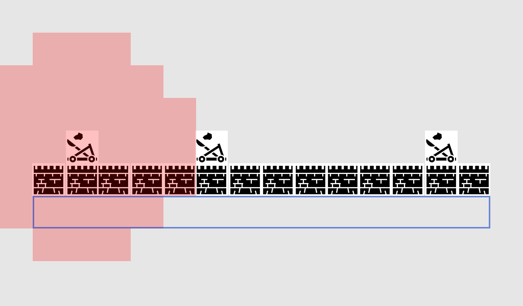
The blue box covers all the squares that we might consider attacking the wall. The red squares represent +1 influence for the catapults, which in this case means somewhere they can attack, and therefore presents danger for an invading unit.

If we now add in the influence from a second catapult:

AI Influence Maps 2.png

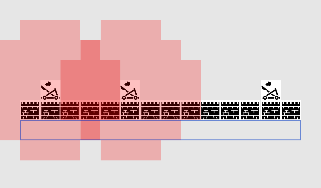
Now we have a darker area, where the influence of the two catapults overlaps, scoring +2 in those squares. The +2 square inside the blue zone would be an especially dangerous place to choose to attack the wall! Let’s add in the influence from our final catapult:

AI Influence Maps 3.png

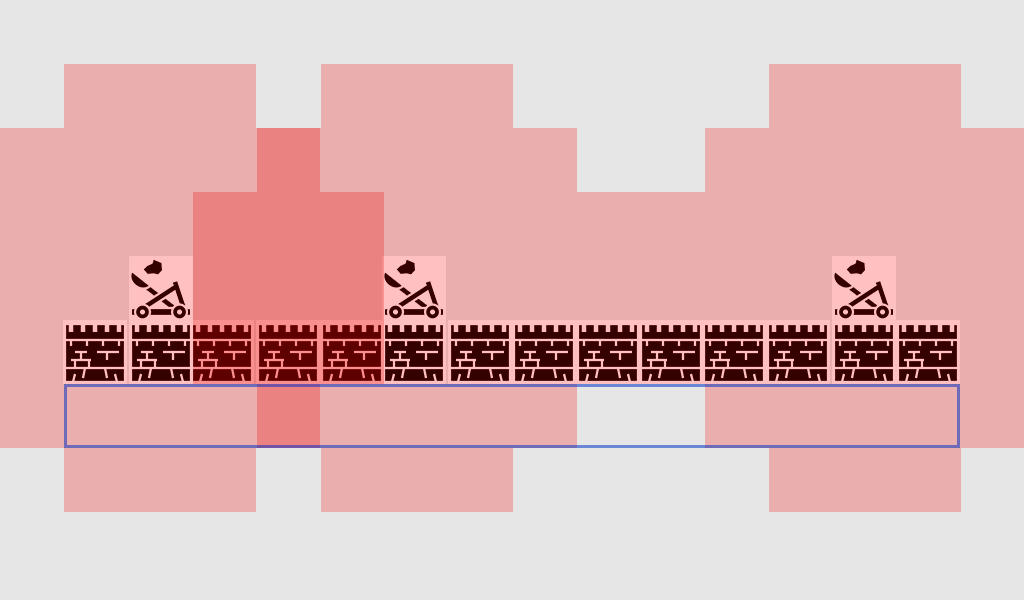
[Icons: CC-BY: https://game-icons.net/heavenly-dog/originals/defensive-wall.html]

Now we have a full indication of the area covered by the catapults. In our potential attack zone, we have one square which has +2 influence for the catapults, 11 squares that have +1, but we have 2 squares which have 0 influence from the catapults – these are prime candidates for our chosen attack position, where we can attack the wall without risking fire from the catapults.

The benefit of the influence map here is that it transforms a continuous space with an almost endless set of position possibilities into a discrete set of rough positions that we can reason about very quickly.

Still, we can get that benefit just by picking a small number of candidate attack positions - why would we choose to use an influence map here instead of manually checking the distance to each turret for each of those positions?

Firstly, the influence map can be very cheap to calculate. Once the map has been written with the influence scores, it doesn’t need to change at all unless the entities in it move. That means you don’t have to perform distance calculations all the time or continue iterating over every possible unit – we ‘bake’ that information into the map just once, and can query it as many times as we like.

Secondly, we can overlay and combine multiple influence maps to perform more complex queries. For example, to find a safe place to flee to, we might take the influence map of our enemies, and subtract the map of our friends – gridsquares with a high negative score would therefore be considered safe.

AI Influence Maps 4.png

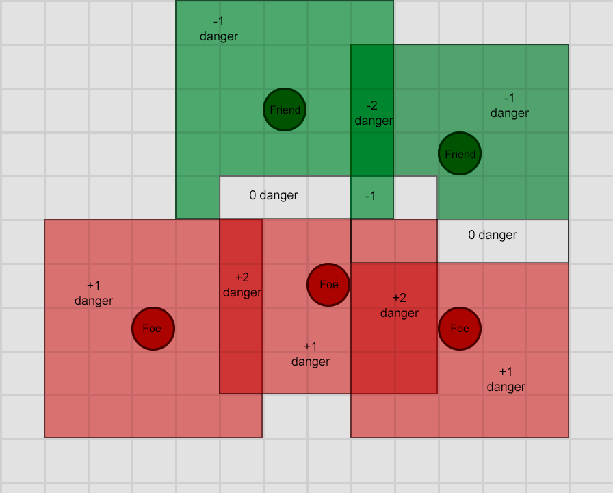
More red means more danger, more green means more safety. Areas where they overlap can fully or partially cancel out, to reflect the conflicting areas of influence.

Finally, they are easy to visualise by drawing them in the world. This can be a valuable aid to designers who need to tune the AI based on visible properties, and can be watched in real-time to understand why the AI is making the decisions that it does.

Conclusion

Hopefully this has given you a broad overview of some of the most common tools and approaches used in game AI, and the situations in which they are useful. Many other techniques - less commonly used but potentially just as effective - have not been covered, and these include:

algorithms for optimization tasks, including hill-climbing, gradient descent, and genetic algorithms
adversarial search/planning algorithms such as minimax and alpha-beta pruning
classification techniques such as perceptrons, neural networks, and support vector machines
systems to handle agent perceptions and memories
AI architectural approaches, such as hybrid systems, subsumption achitectures, and other ways to layer AI systems
animation tools such as motion planning and motion matching
performance considerations such as level of detail, anytime algorithms, and timeslicing

To read more on these topics, and the topics covered in detail above, the following sources may prove useful.

Of course, on GameDev.net you have the Artificial Intelligence articles and tutorials reference as well as the Artificial Intelligence forum.

Here on GameDev.net you have the Artificial Intelligence articles and tutorials reference as well as the Artificial Intelligence forum.
AiGameDev.com contains many presentations and articles about a wide variety of gamedev-related AI topics
The GDC Vault includes the talks from the GDC AI Summit, many available for free: https://www.gdcvault.com/
Similarly, the AI Game Programmers Guild hosts many links to past papers and presentations given at that summit: http://gameai.com/
Tommy Thompson, AI researcher and game developer, has a YouTube channel dedicated to explaining and exploring AI in commercial games: https://www.youtube.com/user/tthompso

Much of the best material can be found in books, including the following:

The Game AI Pro series are collections of short articles explaining how to implement specific features or how to tackle specific problems. Visit http://www.gameaipro.com/ for some free excerpts from the earlier books.
The AI Game Programming Wisdom series are the precursors of the Game AI Pro books, containing slightly older techniques but almost universally still relevant today. Copies are rare so look out for digital copies or bargains!
Artificial Intelligence: A Modern Approach - this is one of the standard texts for anyone wanting to understand the general field of artificial intelligence. This is not a game-specific book, and it can be dense in places, but it gives an unrivalled overview of the area and teaches the fundamentals upon which a lot of game AI is built.

Beyond that there are several good books on general game AI written by industry pros and it would be hard to single any out above the others - read the reviews and pick one that sounds like it would suit you.

Did you like this tutorial? You might also like these other tutorials from GameDev.net's Total Beginner's Guide series:

Are you interested in writing for GameDev.net? Contact us.

[Wayback Machine Archive]

39 Likes 23 Comments

Comments

hero_bash

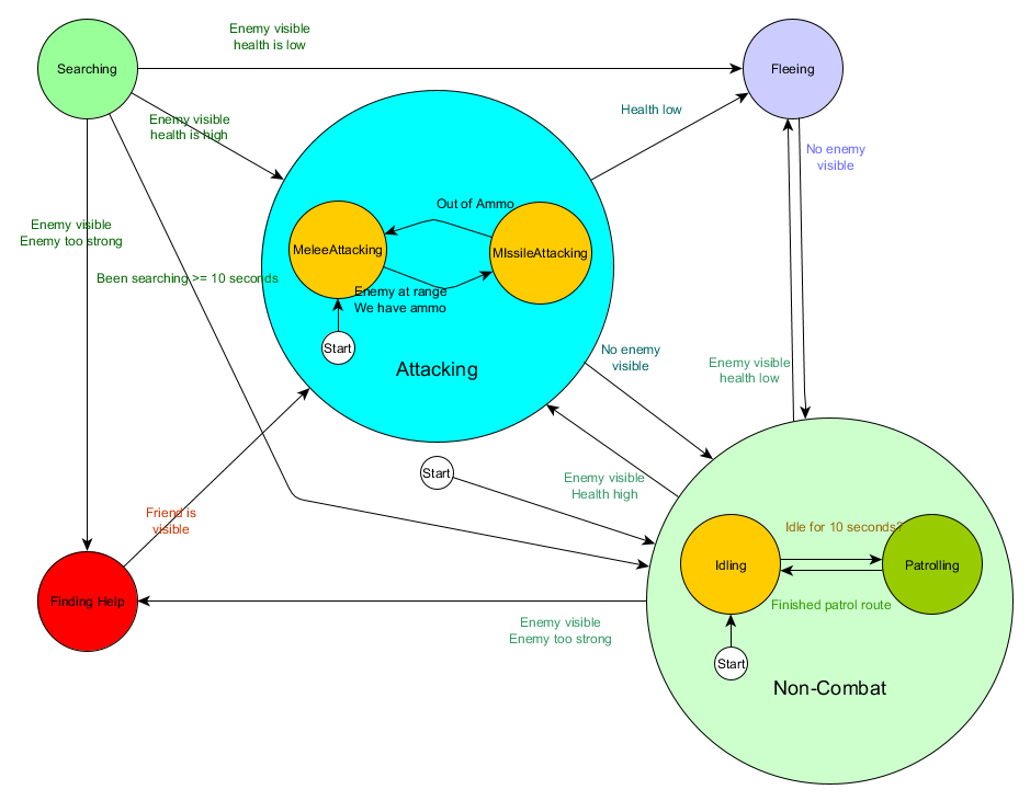
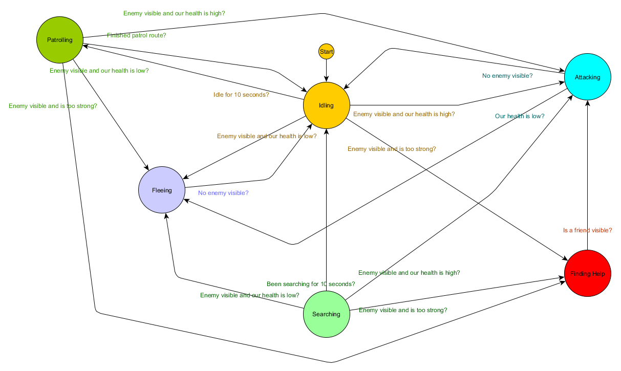
Very comprehensive and informative article. One thing though, the Monte Carlo link takes me to ebay search for listings of Monte Carlo vehicles.

August 13, 2018 07:19 AM

Melodrive

This is an amazing overview! I'd just like to comment on one point regarding the use of neural networks:

Quote

...it’s not practical to write a neural network during development to observe tens of thousands of players and learn the best way to play against them, because the game isn’t released yet and there are no players!

The statement definitely rings true for supervised learning techniques usefdfor training neural nets. However, the late advancements in reinforcement learning could make the use of neural networks feasible also in commercial gaming. Differently from supervised learning, reinforcement learning enables developers to train a neural network without the need of training data. In a reinforcement learning setting, a network can learn by trial and error by running a number of simulations of a game and being exposed to a system of rewards. This approach has been proven to be very successful for developing AI agents that play Atari games, Go and Chess thanks to the work carried out at Deep Mind. Several techniques have been proposed to train networks with reinforcement learning, such as Q-Learning and the use of Genetic Algorithms as a way of evolving the weights and hyper-parameters of a training network. This is definitely exciting research that I'd love to see included in commercial games at some point!

August 13, 2018 11:45 AM

Kylotan

1 hour ago, Melodrive said:

This is an amazing overview! I'd just like to comment on one point regarding the use of neural networks:

The statement definitely rings true for supervised learning techniques usefdfor training neural nets. However, the late advancements in reinforcement learning could make the use of neural networks feasible also in commercial gaming. Differently from supervised learning, reinforcement learning enables developers to train a neural network without the need of training data. In a reinforcement learning setting, a network can learn by trial and error by running a number of simulations of a game and being exposed to a system of rewards. This approach has been proven to be very successful for developing AI agents that play Atari games, Go and Chess thanks to the work carried out at Deep Mind.

This is definitely an interesting area of research, but it is currently focused on playing existing games rather than creating AI for a new game. For the agent to learn by playing the game means you need one of two things:

an existing opponent against which to play - most computer games are too 'asymmetrical' for this approach to work, as a player's goals are very different from the goals of an NPC.
or, a fitness function (such as a high score, or a win/lose condition) which can be used to evaluate the quality of the model - most modern games don't have a suitable measure here that would easily apply to an AI character.

Without these, there are no real rewards with which to reinforce the agent's chosen behaviour, and so this method has limited applicability.

There are definitely applications for reinforcement learning, especially when making opponents for arena-shooters and other symmetrical games such as racing or strategy - and indeed this sort of work has been ongoing since the late 90s, and doesn't necessarily need a neural network architecture to be effective.

August 13, 2018 01:53 PM

Melodrive

4 minutes ago, Kylotan said:

This is definitely an interesting area of research, but it is currently focused on playing existing games rather than creating AI for a new game. For the agent to learn by playing the game means you need one of two things:

an existing opponent against which to play - most computer games are too 'asymmetrical' for this approach to work, as a player's goals are very different from the goals of an NPC.

or, a fitness function (such as a high score, or a win/lose condition) which can be used to evaluate the quality of the model - most modern games don't have a suitable measure here that would easily apply to an AI character.

Without these, there are no real rewards with which to reinforce the agent's chosen behaviour, and so this method has limited applicability.

There are definitely applications for reinforcement learning, especially when making opponents for arena-shooters and other symmetrical games such as racing or strategy - and indeed this sort of work has been ongoing since the late 90s, and doesn't necessarily need a neural network architecture to be effective.

Nice insight, thanks! Unfortunately, I know way to well what it means not to have a fitness function you can rely on for reinforcement learning

My work/research is focused on developing AI systems which generate music. It's quite challenging to find suitable fitness functions which may measure the "goodness" of the generated music, in order to evaluate a generative model. Reinforcement learning - also beyond NNs - is still not really an option in generative music.

On the bright side, I was playing around with deep reinforcement learning in artificial society/life simulations. There, I found the application of RL to be really interesting. With RL, the single agents of a society can evolve very complex behaviours, sometimes unpredictable, without hard-coded instructions. With the "right" reward system, you can end up having emergent behaviour at the level of the super-system. As someone who's really passionate about complexity science, I'm excited to see the (unexplored) possibilities that this technique may open up in this field as well.

August 13, 2018 02:24 PM

Alex Toussaint

On 8/13/2018 at 3:45 PM, Melodrive said:

...it’s not practical to write a neural network during development to observe tens of thousands of players and learn the best way to play against them, because the game isn’t released yet and there are no players!

I did a bit of research in the field (You know I'm something of a scientist myself). I wrote a little Python game (unplayable, just to see the AI's fighting) which uses genetic algorithms and plays a looot of fights to try to find the best weights to outperform the opponent.

I'll leave the link Here in case someone wants to see the code.

So, yes! You can use genetic algorithms to train neural networks to play against humans on very simple games. I believe this approach could be used on more complex games, and even combined with traditional if statements algorithms.

To finish, huge thanks to the authors for its article as huge in quality as in size.

August 14, 2018 03:46 PM

Fulcrum.013

I guess autor have to study a "beginers guide" of AI himslef first . I mean at least university cource of automation control theory, theory of games and theory of descigins.Becouse it imposible to talk about realtime AI without undestending term "real time" and basics of game theory like saddle point theorem.

August 17, 2018 04:29 PM

Locuskidd

Nice write up regarding AI. I'm not sure if I'm really a fan of where games are going as far as artificial intelligence.. as I'm more of a classic gamer, but I'm always open to new things. Can't wait to see what the future holds as far AI and future gaming.

August 17, 2018 04:58 PM

erpeo93

Really good and informative article.

It Covers a lot of things without going in too much details, but then gives study references at the end.

I only consider it to be a bit long, and I probably would have cut it in two parts.

But otherwise, very good job.

Leonardo

August 20, 2018 01:27 PM

rmsgrey

Interesting article, but some aspects of some of the examples ended up distracting me - for example, the FSM has no way of reaching "Searching", which feels like it should be commented on in the text (or corrected in the example). Or, for the Markov model, it appears the sample data was in the form of first sighting and second sighting for independent runs, with second sightings being split 11/14/3 for red/green/blue rooms respectively, which is at odds with the way the data collection was described - as each sighting generating a (last-sighting, current-sighting) pair - which should give the same split of red/green/blue rooms for the next sightings as for the previous sightings (with a possible off-by-one for the boundary conditions).

It would be nice if the examples and the text were more congruent with each other.

August 20, 2018 05:16 PM

kdahlhaus

Thanks - that was a great overview of game AI. It's a good place to start to learn what you might want to learn.

August 22, 2018 01:36 PM

babyjesus

This is amazing. Thank you.

October 22, 2018 02:08 AM

You must log in to join the conversation.

Don't have a GameDev.net account? Sign up!

The Total Beginner's Guide to Game AI

Introduction

What is Game AI?

Constraints of Game AI development

Basic Decision Making

Hardcoded conditional statements

Decision Trees

Scripting

Responding to events

Advanced Decision Making

Finite state machines

Hierarchical State Machines

Behavior Trees

Utility-based systems

Movement and Navigation

Steering

Pathfinding

Movement without a grid

Planning

A Simple ‘Planner’

Improved Planning

Learning and Adapting

Statistics and Probabilities

Basic weight-based adaptation

Markov Models

N-Grams

Knowledge representation

Tags

Smart Objects

Response Curves

Blackboards

Influence Maps

Conclusion

Comments

Featured Tutorial

Recommended Tutorials

Other Tutorials by Kylotan

The Total Beginner's Guide to Game AI

Introduction

What is Game AI?

Constraints of Game AI development

Basic Decision Making

Hardcoded conditional statements

Decision Trees

Scripting

Responding to events

Advanced Decision Making

Finite state machines

Hierarchical State Machines

Behavior Trees

Utility-based systems

Movement and Navigation

Steering

Pathfinding

Movement without a grid

Planning

A Simple ‘Planner’

Improved Planning

Learning and Adapting

Statistics and Probabilities

Basic weight-based adaptation

Markov Models

N-Grams

Knowledge representation

Tags

Smart Objects

Response Curves

Blackboards

Influence Maps

Conclusion

Comments

Featured Tutorial

Recommended Tutorials

Other Tutorials by Kylotan

Reticulating splines