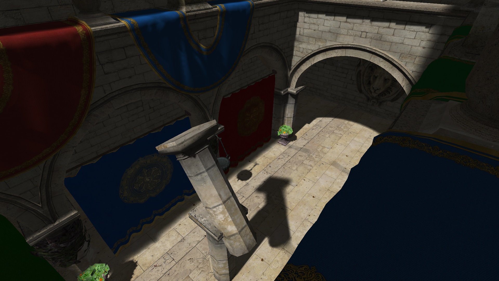
Figure 1: Contact-hardening Soft Shadows in Sponza scene. Note how the green adornments’ shadows are hard (because the shadows are close to the adornments) whereas shadows of poles hanged high in the air (poles are not visible in this screenshot) cast very blurry, barely visible shadows (like on the green adornment in the center of the figure or on the lit wall above the arc). Shadows of the columns in the center of Sponza best present contact-hardening nature of shadows. The content presented here, but from a different point of view, will be a subject of following screenshots. Compare this screenshot with screenshot 2 to better understand which objects’ shadows we will be inspecting throughout the article.
Shadow Mapping [15] is by far the most prevalent technique used to render shadows in real-time. One of its advantages is that it’s quite easy to get decent soft shadows with this technique as in [14]. From that point on we can go straight to contact-hardening soft shadows (CHSS) which was first introduced in Percentage-Closer Soft Shadows (PCSS) paper [7]. [2] reviews the subject extensively.
Soft shadows are slower than standard shadow mapping because they usually require taking more than one shadow map sample, as in aforementioned [14]. There are alternative approaches however – Exponential Shadow Maps (ESM) [6] and Variance Shadow Maps (VSM) [10] – that treat shadow map texels as random variables and apply statistical methods on them. These methods are usually faster but suffer from annoying artifacts like light-bleeding. A completely different approach to producing soft shadows is to blur them in screen space as in [4]. It’s a very interesting approach but comes with all problems associated with computing in screen space – like how to blur a shadow boundary that is covering the entire screen without killing the GPU?
Contact-hardening soft shadows, based on [7], are even slower than regular soft shadows because they require even more samples to look for an average occluder’s depth that is used in estimation of penumbra (region of transition between fully-lit and fully-shadowed areas). So up from barely one shadow map sample we might end up with 16 for occluder’s depth estimation and 32 for actual shadow map filtering. That is a lot by today’s standards, especially having video game consoles in mind. One implementation worth checking out that delivered with a big commerical game is [5].
Statistical methods, like ESM and VSM, and screen space methods both have their merits. In this article however I’ll only focus on how to improve on PCSS. We will start with how to achieve decently big penumbras without the need to take dozens of samples and will proceed on how to make soft shadows contact-hardening at only a fraction of additional GPU time. We will also investigate checkerboarding and see how that relatively new optimization approach performs with regard to shadows rendering.
This article is meant for audience that already has experience in implementing shadow mapping and would like to have fast contact-hardening soft shadows in their games/simulations. This work is heavily based on PCSS [7] and aspires to be its improvement. There is a demo application [11] presenting techniques described here.
Figure 1 presents contact-hardening soft shadows in an actual scenario.
1 Soft Shadows with Few Samples
In order to have bigger penumbra regions a large number of shadow map samples is needed. An initial approach usually involves taking all shadow map samples within a given region. That can be a lot of samples, particularly when the shadow map is of high resolution (for a high-res shadow map, to cover the same world space region, more samples are needed than for a lower-res shadow map, assuming they both cover the same region in world space). A way to speed this up is to use GPU’s sample gather instructions, just like they did in [5] and what is described in [12]. With gather instructions we can reduce the number of sampling operations in a shader four times. But even that might not be enough for big sample kernels that
one might want for elongated soft sunlight shadows.
An alternative to sampling the whole region is to randomly pick a few samples in the region and only use those. But if we take the same random set of samples and apply it to all pixels in the region we will end up with quite nasty banding. Compare figures 2 and 3. To counter this effect we can make sure that each pixel in the region will use a different set of random samples. This will result in noisy shadows, what usually is preferred to banding, but not always. Both have their mertis – noise gives randomness whereas banding gives stability. Ideally we would like something in-between. Turns out that various researchers have worked on this problem and came up with interesting solutions.
We have actually two problems right now to solve. The first one is to figure out what samples to pick for shadow map sampling. The second one is in what way we should pick different samples for different pixels in the region – as we know, using exactly the same samples for all pixels in the region causes banding. We will solve the first problem using Vogel disk samples and the second with interleaved gradient noise.
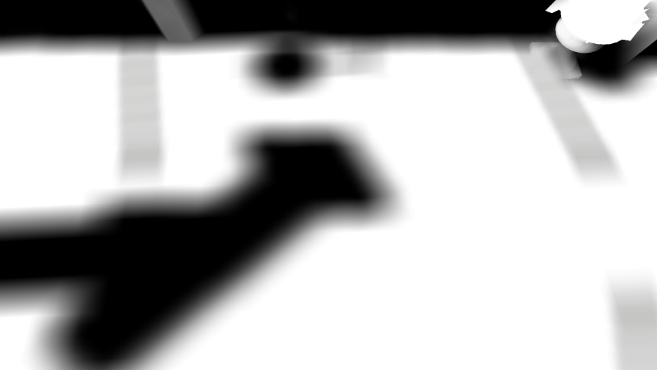
Figure 2: Naive shadows with 11 x 11 kernel, that is 121 samples.

Figure 3: Shadows with 16 samples. Banding is seen because each pixel uses the same shadow map sample coordinates.
1.1 Vogel Disk
Vogel disk algorithm [3] [1] spreads samples on a disk evenly, as shown in figure 4. A great feature of Vogel disk is that when you rotate the points they will never map onto themselves (a given sample will not map onto itself nor any other sample), unless you rotate by 2π.
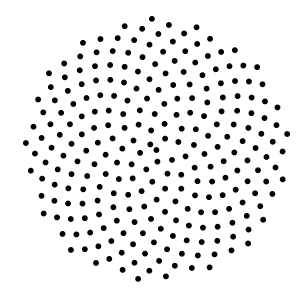
Figure 4: Vogel disk.
Listing 1 shows how to generate Vogel disk coordinates in a shader.
float2 VogelDiskSample(int sampleIndex, int samplesCount, float phi)
{
  float GoldenAngle = 2.4f;

  float r = sqrt(sampleIndex + 0.5f) / sqrt(samplesCount);
  float theta = sampleIndex ∗ GoldenAngle + phi;

  float sine, cosine;
  sincos(theta, sine, cosine);

  return float2(r ∗ cosine, r ∗ sine);
}
Listing 1: Vogel disk samples generation
Alternatively to Vogel disk a somewhat similar set of samples can be generated with blue noise. Blue noise is also often used when not-that-random-randomness is needed, as in [8]. I checked both sets of samples and found that, at least for shadows, Vogel seems to be producing more accurate results with less undersampling. Also Vogel has the advantage that it’s very cheap to compute at runtime. In source code of the demo there is an array declared that stores blue noise samples.
1.2 Interleaved Gradient Noise
Figure 3 actually uses Vogel disk samples for all screen’s pixels but that is not enough to compensate for a low number of samples used. Vogel disk really shines when used in combination with a good random function applied per-pixel. Let’s say that you have a pixels region where each pixel in the region uses the same Vogel disk samples (shown in figure 4) but each pixel applies slightly different rotation to all these Vogel samples, such that this rotation value spans range of [0;2p] for different pixels. This will guarantee that all pixels in the region will sample the shadow map with different sets of samples.
A good random function, called interleaved gradient noise, was developed by [9]. This function takes as input the pixel’s window space coordinates and outputs a "random" number in [0;1] range. Multiplying the result by 2p and passing as argument phi to VogelDiskSample will result in very high quality, very cheap shadows, as presented in figure 5. Usage of interleaved gradient noise is the only difference between the result from figure 5 and 3. Also note how shadows in figure 5 are nicely rounded as compared to squary/blocky in figure 2. The reason for this is that in the latter case a naive 11 x 11 rectangular filter was used.

Figure 5: Interleaved Gradient Noise together with Vogel disk. Only 16 shadow map samples.
Listing 2 presents interleaved gradient noise function.
float InterleavedGradientNoise(float2 position_screen)
{
  float3 magic = float3(0.06711056f, 0.00583715f, 52.9829189f);
  returnfrac(magic.z * frac(dot(position_screen, magic.xy)));
}
Listing 2: Interleaved Gradient Noise
2 Contact-hardening Soft Shadows
In this section, we will see how contact-hardening shadows work, as presented in [7]. After that, we will go through two different ways that speed up the base algorithm.
2.1 Regular Solution
To add contact-hardening’ness to soft shadows all we need is to know how big penumbra for a given pixel is, or in other words, how big the shadow map sampling kernel for a given pixel should be. This is estimated with a procedure called average blocker search shown in figure 6. We have a receiver, whose little red square is the pixel we’re calculating shadows for. There is also a blocker floating above the receiver that blocks some light and finally a light source (and its shadow map). We need to find depths (in light space) of pixels that block the red square from light, average those depths and use that average to compute size of penumbra in that area.
Think about what this particular shadow map from figure 6 contains. The right side of that shadow map contains depths of the blocker, whereas the left side stores the blue receiver’s depths. If we take some kernel around the receiver’s red area and take a few samples (orange dots) to sample the shadow map some of those samples will sample the blocker’s depths (samples that are on the right side) and some will sample the receiver (samples that are on the left side). Since the red area’s depth is more or less equal (up to some bias that we usually employ in shadow mapping techniques) to the depths to the left we don’t consider them (those depths) as blockers. But we do treat as blockers depths that are smaller (closer to the light) than the depth of the red area, which in this case are depths that come from the green blocker. These depths, from the green blocker, are averaged together to yield average occluder’s depth that will let us estimate pixel shadow’s penumbra.
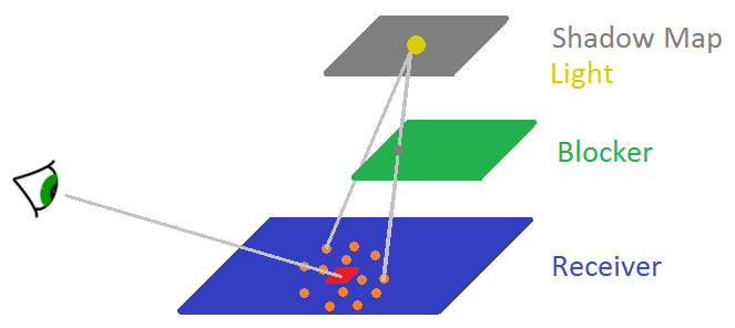
Figure 6: Average blocker search. Orange dots/samples’ depths are checked against depths in the shadow map.
Shadow map’s depths that are closer to the light are considered blockers and are averaged together.
It is important to realize that this algorithm has its drawbacks. Look again at figure 6 and the blocker.
Now imagine you have not one but two such blockers where one of them (call it b1) is very close to the light source and the second one (call it b2) is very close to the receiver. Since shadow map only stores depths of the closest layer, that is blocker b1 in this case, it has no information about blocker’s b2 depths. And it is blocker b2’s depths that we care about in this case. This is where average blocker search based on only one-layer shadow map will fail. An obvious solution to this problem would be to store more layers of depths in the shadow map but that would be an overkill. Fortunately, artifacts that are the result of this drawback are often negligible.
Listing 3 shows a function that calculates penumbra, which is a value used to scale shadow map sampling kernel.
float Penumbra(float gradientNoise, float2 shadowMapUV, float z_shadowMapView, int samplesCount)
{
  floatavgBlockersDepth = 0.0f;
  floatblockersCount = 0.0f;

  for(int i = 0; i < samplesCount; i ++)
  {
    float2 sampleUV = VogelDiskOffset(i, samplesCount, gradientNoise);
    sampleUV = shadowMapUV + penumbraFilterMaxSize * sampleUV;

    floatsampleDepth = shadowMapTexture.SampleLevel(pointClampSampler, sampleUV, 0).x;

    if(sampleDepth < z_shadowMapView)
    {
      avgBlockersDepth += sampleDepth;
      blockersCount += 1.0f;
    }
  }

  if(blockersCount > 0.0f)
  {
    avgBlockersDepth /= blockersCount;
    return AvgBlockersDepthToPenumbra(z_shadowMapView, avgBlockersDepth);
  }
  else
  {
    return 0.0f;
  }
}
Listing 3: Penumbra calculation.
Function Penumbra first finds average blockers depth and then converts that value to actual penumbra with AvgBlockersDepthToPenumbra.
Listing 4 shows the implementation of that function.
float AvgBlockersDepthToPenumbra(float z_shadowMapView, float avgBlockersDepth)
{
  float penumbra = (z_shadowMapView - avgBlockersDepth) / avgBlockersDepth;
  penumbra *= penumbra;
  return saturate(80.0f * penumbra);
}
Listing 4: Average blockers depth to penumbra conversion.
This function should be implemented such that it suits your needs.
The basic idea is to take the distance between pixel we’re calculating shadows for z_shadowMapView and average blockers depth. The bigger that distance is the bigger the penumbra should be. In case of the demo accompanying this article, depths are all in shadow map’s view space. The 3rd line of code calculates the distance and "normalizes" it. Later on, we square it to get rid off of possible minus sign but also to make a more visible transition between fully-hard and fully-soft shadows. Finally, the penumbra is scaled by some constant and brought down to [0;1] range.
The original formula from [7] is a bit different from listing 4 and takes light’s size into account directly, making it more physically correct. It is shown in listing 5.
float AvgBlockersDepthToPenumbra(float lightSize, float z_shadowMapView, floatavgBlockersDepth)
{
  float penumbra = lightSize * (z_shadowMapView - avgBlockersDepth) / avgBlockersDepth;
}
Listing 5: Average blockers depth to penumbra conversion from [7].
You should fiddle with that function to get the look and feel of soft shadows and hard-to-soft transition that accomodates your needs.
For the sake of completeness listing 6 shows how penumbra estimation function is used in conjunction with actual shadow map sampling.
float penumbra = Penumbra(gradientNoise, shadowMapUV, z_shadowMapView, 16);

float shadow = 0.0f;
for(int i = 0; i < 16; i++)
{
  float2 sampleUV = VogelDiskOffset(i, 16, gradientNoise);
  sampleUV = shadowMapUV + sampleUV * penumbra * shadowFilterMaxSize;

  shadow += shadowMapTexture.SampleCmp(linearClampComparisonSampler, sampleUV, z_shadowMapView).x;
}
shadow /= 16.0f;
Listing 6: Shadows computation with penumbra used as kernel scale.
In line 9, instead of using traditional shadow mapping by sampling shadow map and comparing depths, we use function SampleCmp together with linearClampComparisonSampler sampler to let hardware take four closest samples, compare them all and bilinearly filter the results. This is much faster than doing that in the traditional way.
Figure 7 presents contact-hardening soft shadows in action.
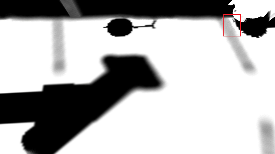
Figure 7: Regular contact-hardening soft shadows. We clearly see how far from the ground objects are. The red rectangle indicates an area with shadows with highly varying penumbra size hence some jittering/jaggies can be seen. These jaggies are caused by the fact that some pixels (randomized by interleaved gradient noise) fall in areas of zero penumbra and some in areas of maximum penumbra hence varying lightness/shadowness of pixels.
2.2 Penumbra Mask
Penumbra estimation, if uses the same number of samples as actual shadow mapping, can be equally expensive as actual full soft shadow mapping. So the cost of contact-hardening soft shadows is twice as big in this case. Lowering the number of samples by half (only for penumbra) can significantly reduce rendering time. It will still be a few dozens percent slower than full non-contact-hardening soft shadows though. The simplest way to significantly reduce rendering time is to apply the same trick that we use all the time in real-time rendering – render at lower resolution.
Shadows themselves need full-screen resolution because they are very high frequency phenomenon (there are rapid changes in intensity of the signal – there is a shadow of an object for a few pixels and then suddenly there can be a fully lit area, with shadow ending abruptly). But penumbra is actually changing gradually quite often so it is a good candidate for rendering at lower res and then upsampling the results. In essence, we split the shadow mask generation pass in two passes: first one that computes penumbra mask at quarter res (penumbra mask pass) and second that computes actual soft shadows but samples penumbra from the penumbra mask (shadow mask pass).
Figure 8 shows the result of that change.
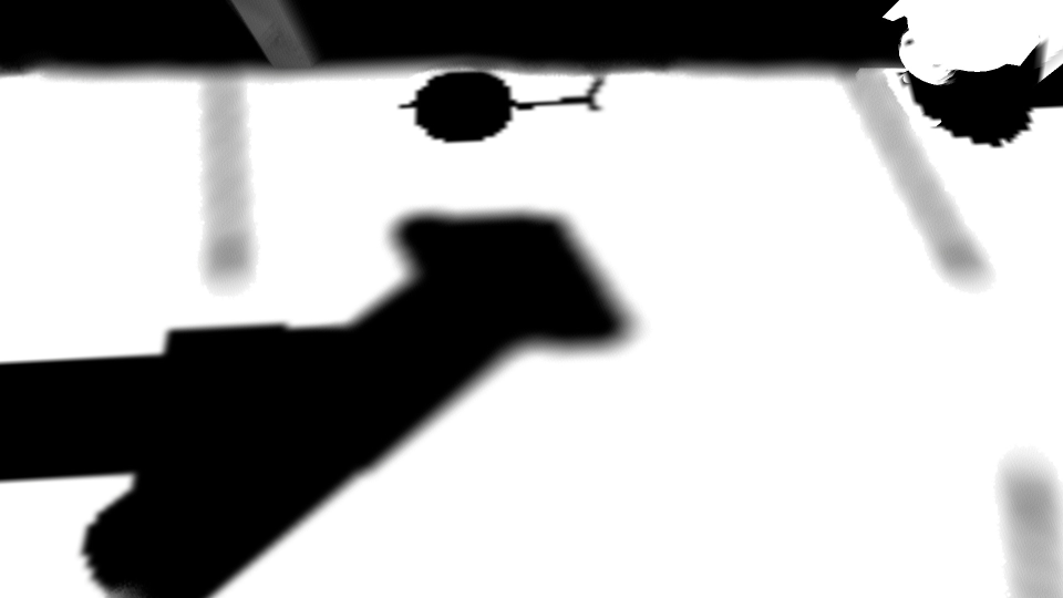
Figure 8: Soft shadows with penumbra rendered in a separate pass in lower res.
As you can see it’s quite nice with the exception that penumbra often ends abruptly (look at those oblong poles’ shadows). If we look at how upsampled (bilinearly) penumbra mask looks like we will understand why (figure 9). We have for instance areas with maximum penumbra (white color), interleaved with zero penumbra areas (black color). The problem was there before but because we rendered in full res interleaved gradient noise was equally good for sampling for both shadows and penumbra. Now that we render penumbra in lower res it is not enough. Not all is lost though. A simple solution is to increase penumbra’s sampling kernel’s size. Multiplying by 1:2 (with regard to what is used for actual shadow mapping) will result in what is seen in figure 10.
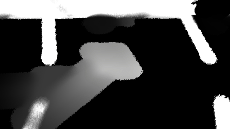
Figure 9: Penumbra mask visualized.
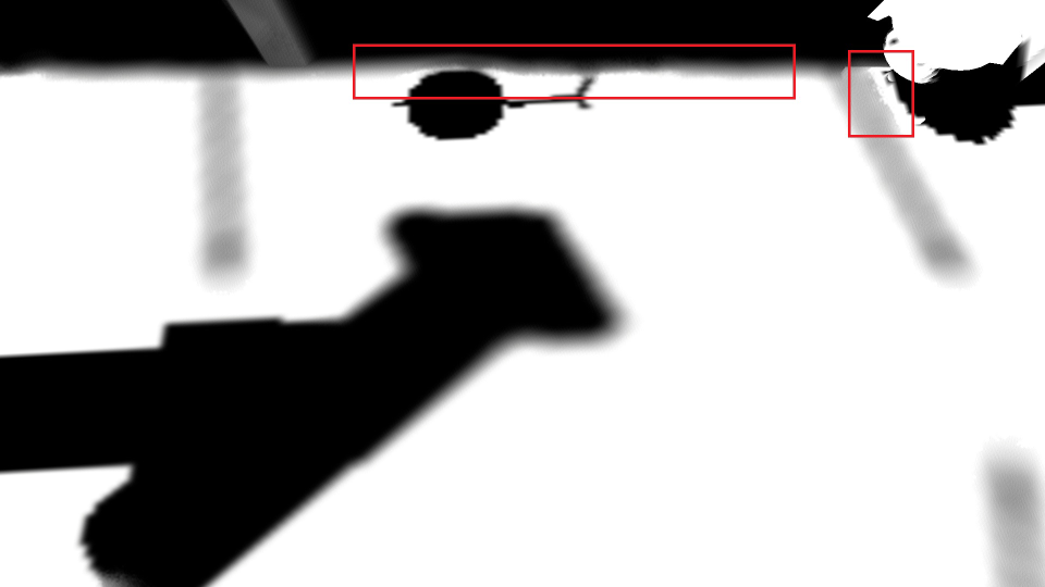
Figure 10: Soft shadows with penumbra rendered in a separate pass in lower res using kernel scaling trick. The red rectangles outline the same types of areas that were described in caption of figure 7. This time, because we’re rendering in lower res and upsample, jittering is more obvious and looks like sort of bubbles (despite the kernel scaling trick). It wouldn’t be a big problem if it wasn’t for a fact that very distracting swimming occurs under camera motion.
Figure 10’s caption describes problem with swimming bubbles – even though we scaled the kernel it is not enough to eliminate all artifacts. We need another hack to fix this. The solution is to blur the penumbra mask to sort of soften the bubbles. Figure 11 shows how penumbra mask looks like when blurred with 7*7 separable Gaussian blur with s = 3. Figure 12 shows the final result of both applying kernel scaling and blurring the penumbra mask.
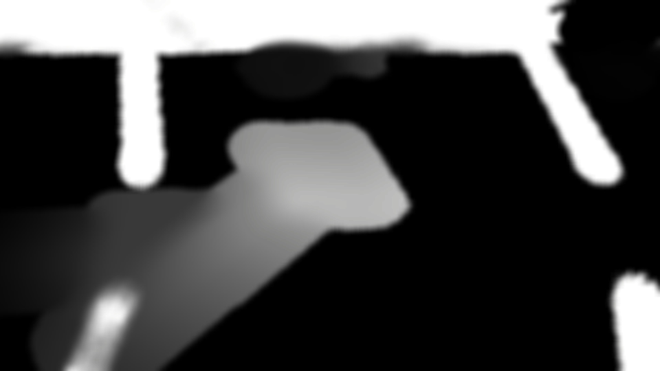
Figure 11: Penumbra mask blurred visualized.

Figure 12: Soft shadows with penumbra rendered in a separate pass in lower res. Kernel scaling of 1:2 for penumbra estimation applied. Also, penumbra mask used is blurred with 7*7 separable Gaussian blur with s = 3.
If you have an eye for detail you will notice that the problem we had before, with abruptly ending penumbra, has been reintroduced somewhat (compare shadow of a post on the left). It’s not as bad as in figure 8 but little worse than in figure 10. So why is it back exactly? Because we blurred the penumbra mask and thus made zero-penumbra regions to bleed onto full-penumbra regions. We can fix this again by simply scaling penumbra kernel by more than 1:2. Of course, we cannot increase that scale indefinitely as at some point penumbra estimation will start to miss occluders and the result will not be conformant with what the shadow mask pass is sampling. But there are values in range about [1:2;1:6] where the vast majority of artifacts is gone.
Blurring penumbra mask introduces two other problems that don’t necessarily need to be fixed for the effect to look good but it’s worth knowing about them.
As we know, penumbra mask is calculated in lower res in screen space. We blur it to alleviate artifacts that stem from rendering in low res. But because we’re working in the camera’s screen space, blurring "just like that" will make penumbra mask to bleed/blend between geometries that are at possibly very different depths/distances from the camera. This is a huge problem for screen space effects like screen space ambient occlusion where they are immediately seen. But it turns out this is almost no problem for penumbra mask computation. If you want you can do smart blurring by sampling the depth buffer and compare depths but that is really not necessary in my opinion.
Another problem is a bit more annoying. Because we blur in screen space with a constant-size kernel, the farther away the camera goes from a shadow, the more penumbra blurring kicks in. This will have the effect of decreasing penumbra size for shadows that are far away from the camera (making soft shadows harder). To fight this just scale penumbra blur kernel using the distance from pixel to the camera, just as it is used in effects like screen space ambient occlusion. Note that this solution is not implemented in the demo application, but I quickly prototyped it locally and found it to work as expected.
Penumbra blurring is a must to avoid swimming bubbles. But it is possible to avoid blurring in of smaller values onto bigger values (this effect decreases penumbra size). Before blurring the penumbra mask with 7*7 kernel you can first use 7*7 max filter. These two, max and blur combined, will have the effect of only blurring outwards so no bigger values will ever be washed out by smaller ones. This idea actually sounds better than it works. The problem is that max filter loses information, penumbra information in this case, and this leads to a lot of subtle artifacts. Hence I’m not recommending using that filter. I’ve tried a multitude of combinations of max and Gaussian blur filters and always retracted to one single Gaussian blur pass. Also due to performance reasons.
There is actually one more alternative solution to drawbacks that blurring of the penumbra mask brings. Look at listing 3, line 27. Now, look at figure 9. As you can see, when a pixel is fully lit, i.e. it does not have any occluders, we return 0. But what if we returned 1 instead? The pole’s (on the left) penumbra would not be affected by blurring at all and that shadow would look correct regardless of distance of a pixel from the camera. At least, in this case, it would be all fine. In other cases, we would have reversed artifacts. Earlier our problem was that distant shadows that should be soft would become hard. Here it would be the opposite – distant shadows that are hard would become soft. Unless we scaled Gaussian blur kernel according to pixel’s distance from the camera of course.
One more important property of outputting 1 by default instead of 0 is that scaling the kernel in penumbra
mask pass is no longer necessary. So in the end you might prefer to output 1 on default.
There has been a lot of dicussion about problems related to rendering penumbra in a separate pass in lower res and how to fix them. Let’s now sum things up. To get contact-hardening soft shadows we need to know what penumbra a pixel has. To calculate penumbra fast we need to do it in a pass separate from shadow mask because we can do it in lower resolution as penumbra is rather low frequency phenomenon. When we do so, things generally work except for some artifacts. To fix those artifacts it is usually sufficient to blur the penumbra mask and increase kernel size when sampling the shadow map in the penumbra mask pass. The latter is not necessary if penumbra mask outputs 1 instead of 0 on default.
At this point, you should have nice contact-hardening soft shadows that are almost as fast as non-contacthardening soft shadows. There is one last problem though that I wasn’t able to solve. Again, because we’re rendering penumbra in low res and we also blur it, there are some shadows swimming where areas with highly varying penumbras blend. This usually is a problem if you use too small shadow map for too big scene’s area. But that is something you usually avoid by using cascade shadow mapping for instance. So all in all little shadows swimming that is left in those situations can be neglected.
2.3 Min Filter
Before I ever came up with an idea of penumbra mask I first came with an idea of using a min filter on a shadow mask. This solution is not appealing to me today but I wanted to mention it. It is implemented in the demo application but it’s turned off "hardcodingly" so you need to fiddle with the source code to be able to turn it on.
In standard CHSS we first find average blocker’s depth. Since that is expensive part of the algorithm I looked for ways to speed this up, even if they are only approximations. I came up with an idea to, instead of finding average blocker’s depth, use minimum depth from the shadow map over some texels region (region of max penumbra size of course). In average blocker’s depth we sample a bunch of texels, say in a 5*5 shadow map’s region, to see if they are closer to the light source than the pixel we’re calculating penumbra for; those that are closer to the light source are averaged together. The idea of min filter is to just take a single min value over the whole filter region 55 and use that directly instead of the average blocker’s depth. The reason why min filter makes sense is that this value will always be closer to the light source than the pixel we’re calculating penumbra for. So it is some kind of blocker’s depth. Not very sophisticated and rather crude one but still.
But why would you do that if you can just compute the average? Because applying min filter over a region does not require from us doing it in the shadow mask pass. We can compute min shadow map over a shadow map in a separate pass. Moreover, min filter is a separable filter, which means we don’t have to take n2 samples (assuming n*n region) but we can do two passes, horizontal and vertical, each requiring n samples, totalling 2n. We traded quadratic complexity (dependent on the screen’s resolution) for linear complexity (dependent on shadow map size).
One problem with the min filter is that, by its nature, it loses a lot of information. It will create lumps of pixels, with all pixels in a lump having the same depth, and these depths will often differ significantly. A solution to that is to blur the min shadow map. Later, in the shadow mask pass, you simply sample the blurred min shadow map and use that instead for the average blocker’s depth. Blurring the min shadow map will have the effect of pushing those min values a bit towards pixels, farther from the light source, what could possibly push them behind pixels that use them (an "occluder" ends up being behind a pixel). In practice, however, that is not a problem.
Figure 13 shows the results. Compare that to figure 12. One change is in round shadows of an adornment in the top middle part of the figure. Figure 12 handled that nicely whereas in figure 13 we see how min depth from some distant geometry is flooding neighbours, including the adornment, and makes its penumbra very large. Another problem occurs on the shadows of a column that is spread from the left to the center of the figures. Both the top pole’s min depth is flooding the column as well as some distant geometry on the bottom
left of the picture, both making the column’s shadows in the middle very penumbra-large.

Figure 13: Soft shadows with penumbra calculated using min filter applied to shadow map.
So we know min filter kind of sucks. Does it have any advantages over solution we discussed in the previous section? Yes. Because min filter works in shadow map’s space and not in screen space we don’t have any swimming artifacts under camera’s motion. That is a nice feature of that algorithm as it makes it more stable.
3 Checkerboarding
Since the advent of "even more next-gen" consoles like PS4 Pro developers decided to aim even higher in terms of quality and try touching the magical 4k barrier. PS4 Pro indeed has measurably more computing power than bare bones PS4 but not enough to pull off 4k just like PS4 handled full HD. So developers resorted to kind of cheating to achieve 4k with only half of the power available. To checkerboarding.
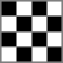
Figure 14: Checkerboard pattern.
Look at figure 14. The idea of checkerboarding is to perform calculations only every other pixel in checkerboard pattern. This way we only need half of computing power. The missing pixels are then filled in some way. The tricky part is figuring out this "some way". The way that is implemented in the demo is by averaging the neighbours. Take a look at the figure again. Assume black pixels represent those for which we calculate shadows. Now think about one of the white pixels, which is not computed. The idea of averaging is to simply take the four neighbouring black pixels, average them and plug that value into the white pixel. There is one catch though. The neighbours might belong to different geometries and since shadows are rather a high-frequency phenomenon (as opposed to penumbra) averaging them thoughtlessly will end up in artifacts. To do it right we need to perform depth comparisons of the neighbours with the pixel we’re averaging for and only blend in those neighbours whose depths don’t differ much – it’s the very same way we do it when performing bilateral upsampling in many postprocessing algorithms to save on computing power, like SSAO or depth of field.
Alternatively, instead of computing averages we could employ temporal filtering and flip the checkerboard pattern every second frame. This should result in shadows quality being on par with full res shadow mask.
If you have ever tried computing a high-frequency signal in low res and then upsample it you know that this just does not work well. It’s hard to make SSAO stable, which is quite low-frequency effect, let alone shadow mask. That is true when the low res we are talking about means computing in a buffer which is half of the screen’s width in width and half of the screen’s height in height, or in other words four times smaller. In this scenario problems are mostly visible at oblique angles. When the camera is looking straight ahead on a wall with some even-not-that-smooth-shadows it’s okay. But once the camera is at an oblique angle to some floor, swimming artifacts appear, stemming from undersampling, and they are extremely distracting. You might increase the resolution of the low res buffer such that overall it is twice the size of the screen’s resolution but that will not eliminate the problem – swimming will remain, although it will be reduced a bit.
If instead of trying to squeeze as much as possible from rendering in low res and upsampling you will render in full res but in checkerboard pattern, what requires only half of memory and computing only half of the pixels, you will find out that the swimming problem at oblique angles is completely gone. That is the most powerful feature of this algorithm. There will still be some minor swimming artifacts in very detailed areas of the screen where you just don’t have that info you would have had if you had stayed in standard full res but there are high chances that the result will be good enough.
Truth to be told, there is a little lie in statement that checkerboarding costs half as much as full res path. Checkerboarding requires smart upsampling, which includes sampling the depth buffer, and that costs some time. This pass’s time is however constant. So the more expensive the checkerboard res computation pass the less, relatively, upsampling costs.
Checkerboarding is supported in the demo application. The application creates a separate render target for storing results of checkerboarded shadow mask. This render target is of height the same as the screen’s height but with half the width. Checkerboard-computed pixels are "packed" into this buffer and later, in the upsample pass, unpacked. Also, the missing pixels are filled in (interpolated). Source code that handles checkerboarded shadow mask in shaders is located in two places. First, there are some minor modifications
to the shadow mask pass itself to handle checkerboarding. The second place is a dedicated shader that performs upsampling. The code is rather easy to follow. One important change is in the gradient noise formula in the shadow mask pass. Using the original formula made samples look less random than in full res. I experimented with the formula and found one modification to work reasonably well but I think that one could come up with a more scientific-based formula. Let’s now see the only modification to the shadow mask shader code, presented in listing 7.
float2 CheckerResPixelCoordToFullResUV(int2 pixelCoord)
{
  pixelCoord.x *= 2;
  if(pixelCoord.y % 2 == 1)
  pixelCoord.x += 1;
  return((float2)pixelCoord + float2(0.5f, 0.5f)) * screenPixelSize;
}

. . .

#ifndef USE_CHECKER
  float2 uv = input.texCoord;
  float gradientNoise = TwoPi * InterleavedGradientNoise(uv * screenSize);
#else
  float2 uv = CheckerResPixelCoordToFullResUV(pixelCoord);
  floatgradientNoise = TwoPi * InterleavedGradientNoise(uv * screenSize * float2(1.0f, 4.0f));
#endif
Listing 7: Checkerboarding in the shadow mask shader.
As you can see the only modification to the interleaved gradient noise function is multiplication of the y-coordinate by 4.
In the upsampling shader a few optimizations can be turned on/off via defines what can make the shader harder to follow but it really does no magic. One of the optimizations is using 16-bit floating-point (linear) depth buffer. Second and third ones, more important, involve using GatherRed instructions, both on the shadow mask and the depth buffer (both are one-channel textures), to save on sampling instructions.
Figure 15 shows checkerboarded shadow mask in action. With careful eye inspection one can indeed see that the dithered smooth shadows are a bit more crude in the checkerboard variant.

Figure 15: Shadow mask calculated in checkerboard resolution and upsampled.
4 Demo
As it was already mentioned there is the demo application accompanying this article. It is implemented using framework MaxestFramework [13] and uses Direct3D 11 as rendering API. It is located in [11].
Key configuration:
- WSAD + mouse – camera movement.
- Shift – speeding up.
- Space – aligns the light direction with the current camera’s view vector.
- Q – if pressed it will display penumbra mask.
- E – if pressed penumbra mask blurring is turned off, what will let see bubbles artifacts.
- F4 – recompile shaders.
- ESC – exit.
The demo’s HUD displays a multitude of various options to turn on/off and tweak.
4.1 Performance Comparison
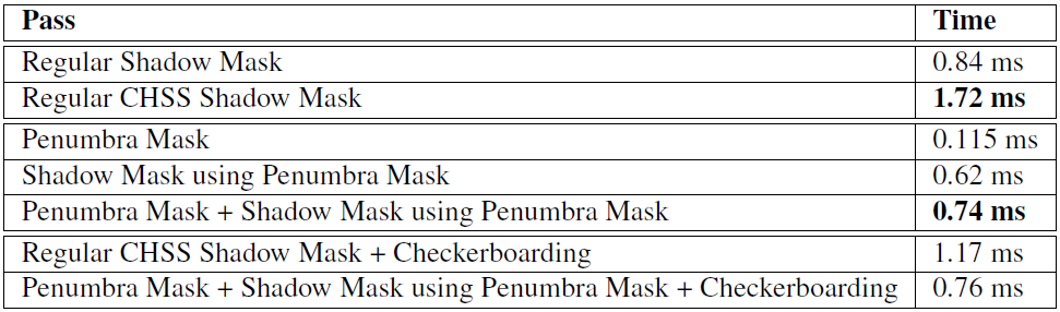
Table 1: Performance on GeForce 660 GTX in 1080p and 20482 shadow map resolution. All shadow mask passes take 16 samples. Penumbra Mask takes 32 samples.
Table 1 shows exemplary performance comparisons for the view presented in the screenshots shown throughout the article. Note here that penumbra pass takes two times more samples (32) than the shadow mask pass (16) while in the original paper [7] this proportion was reversed. One reason is that in this demo we use hardware bilinear shadow map samples filtering so in the end we are not using 16 shadow map samples but actually 64. Another reason is that we could in fact use a smaller number of samples for penumbra, like 16, and this works good but only in the original PCSS implementation. When using penumbra mask pass with only 16 samples then some small artifacts start to pop up. I found 32 samples to work good in quarter res of penumbra mask pass and 16 to be okay for original PCSS. The demo lets you switch between 16 and 32 samples used in penumbra estimation to see the difference.
Regular Shadow Mask is a pass that uses no contact-hardening and whose results are shown in figure 5. Next, there is Regular CHSS Shadow Mask whose results are in figure 12. CHSS is roughly two times more expensive than no-CHSS approach. Note here that penumbra pass takes 32 samples whereas shadow mask takes 16. That would imply that Regular CHSS Shadow Mask should be more than two times as expensive as Regular Shadow Mask. It’s not because as you can see in figure 12 most shadows have low penumbras, thus shadow map sampling kernels are not wide. In case where shadow map sampling kernels of all screen’s pixels are maxed the performance difference would be greater.
Now going to the gist. Performance measurements for Shadow Mask using Penumbra Mask clearly depict great performance boost. Together with Penumbra Mask both these passes jointly take 0:74 ms what is more than two times faster than Regular CHSS Shadow Mask pass at 1:72 ms. The reason for that is that in Regular CHSS Shadow Mask most performance hit comes from penumbra estimation (32 shadow map samples) and this part is what has been optimized. Note that performance of Penumbra Mask + Shadow Mask using Penumbra Mask (0:74 ms) is even better than Regular Shadow Mask’s (0:84 ms). The reason for that surprising difference is obviously that for a tested scene most screen’s pixels in penumbra variant have small shadow map sampling kernels and that is what is mostly responsible for great performance. However, in situations where the whole screen is filled with max-penumbra pixels the performance of Penumbra Mask + Shadow Mask using Penumbra Mask is only about 10-15% worse than in Regular Shadow Mask pass.
Finally, checkerboarding indeed is capable of speeding up Regular CHSS Shadow Mask. It does not perform well when we use penumbra mask though. The reason is that Shadow Mask with Penumbra Mask pass becomes so cheap that checkerboarding-related operations like upsampling become very expensive, relatively. The take-away for checkerboarding is to use it only when the pass that it is optimizing is relatively expensive.
4.2 Future Work
This work can further be improved, both on the penumbra generation side as well shadow mask.
Using penumbra mask greatly improves performance but comes with some swimming artifacts which might or might not be a problem. Possibly using temporal filtering could help here. Instead of rendering penumbra mask in quarter res we could still render in full res but only compute one pixel in a 2*2 quad, filling the remaining pixels in subsequent frames. Given that penumbra mask contains low-frequency data this could work.
When it comes to shadow mask it could be beneficial to use more than one mipmap of the shadow map. This would be just for efficiency purposes. By increasing filtering radius we induce more performance hit due to texture cache misses. For samples that are farther we could sample the second mipmap of the shadow map. This applies to penumbra mask as well.
Implementation of temporal checkerboarding is also tempting. Quality should be comparable to full res shadow mask and performance increase should be significant. This could be particularly desirable if we needed more shadow map samples.
5 Conclusions
The point of this article was to present an efficient way to render contact-hardening soft shadows, based on original idea from [7]. I believe that separation of penumbra estimation (in lower res) and shadow mask rendering is the way as it allows for achieving performance nearly as good as when rendering regular soft shadows. There is a cost in form of some swimming artifacts which should not be a deal-breaker. The overall image quality boost that CHSS brings is at least worth exploring, given that performance with regard to non-CHSS will suffer only a tiny bit with penumbra mask approach.
In this paper we discussed:
- Efficient soft shadows with Vogel disk and interleaved gradient noise.
- Original PCSS implementation.
- Penumbra mask as a way to decouple penumbra estimation from shadow mask generation to greatly improve performance.
- Min filter as another way to decouple penumbra estimation from shadow mask generation. Worse quality and performance than in penumbra mask approach though.
- Use of checkerboarding with shadow mask generation.
6 Acknowledgments
I would like to thank Krzysztof Narkowicz of Epic Games for proofreading this article and Adam Cichocki of Microsoft for his ideas to use Vogel disk and checkerboarding.
References
[1] 4rknova. Shadertoy: Vogel’s Distribution Method. https://www.shadertoy.com/view/XtXXDN.
[2] Louis Bavoil. Advanced Soft Shadow Mapping Techniques. http://gamedevs.org/uploads/advanced-soft-shadow-mapping-techniques.pdf.
[3] Alexandre Devert. Spreading points on a disc and on a sphere. http://blog.marmakoide.org/?p=1.
[4] Marton Tamas et al. Chapter 4.1 in GPU Pro 6: Practical Screen Space Soft Shadows. https://www.crcpress.com/GPU-Pro-6-Advanced-Rendering-Techniques/Engel/p/book/9781482264616.
[5] Peter Sikachev et al. Chapter 2.1 in GPU Pro 6: Next-Gen Rendering in Thief. https://www.crcpress.com/GPU-Pro-6-Advanced-Rendering-Techniques/Engel/p/book/9781482264616.
[6] Thomas Annen et al. Exponential Shadow Maps. http://citeseerx.ist.psu.edu/viewdoc/download?doi=10.1.1.146.177&rep=rep1&type=pdf.
[7] Randima Fernando. Percentage-Closer Soft Shadows. http://developer.download.nvidia.com/shaderlibrary/docs/shadow_PCSS.pdf.
[8] Mikkel Gjol and Mikkel Svendsen. The Rendering of Inside. https://github.com/playdeadgames/publications/blob/master/INSIDE/rendering_inside_gdc2016.pdf.
[9] Jorge Jimenez. Next Generation Post Processing in Call of Duty: Advanced Warfare, 2014. http://www.slideshare.net/guerrillagames/killzone-shadow-fall-demo-postmortem.
[10] Andrew Lauritzen. Summed-Area Variance Shadow Maps. https://developer.nvidia.com/gpugems/GPUGems3/gpugems3_ch08.html.
[11] Wojciech Sterna. Contact-hardening Soft Shadows Demo. https://github.com/maxest/MaxestFramework/tree/master/samples/shadows.
[12] Wojciech Sterna. DirectX 11, HLSL, GatherRed. http://wojtsterna.blogspot.com/2018/02/directx-11-hlsl-gatherred.html.
[13] Wojciech Sterna. MaxestFramework. https://github.com/maxest/MaxestFramework.
[14] Yury Uralsky. Efficient Soft-Edged Shadows Using Pixel Shader Branching. https://developer.nvidia.com/gpugems/GPUGems2/gpugems2_chapter17.html.
[15] Wikipedia. Shadow mapping. https://en.wikipedia.org/wiki/Shadow_mapping.
About the author:
Wojciech has over 6 years of professional engine/technology/game programming experience, with strong C++ and graphics/rendering emphasis, enriched with experience in
other areas including multiplatform, multithreaded and multiplayer programming, high-performance computing (GPGPU) and machine learning (first steps here). Wojciech is keen on
understanding mathematical and/or algorithmic fundamentals of tools he uses.
This paper was originally published on the author's homepage and is reproduced here with kind permission.


Hey,")

the book you wrote on OpenGL was the first graphics book I read
I'm doing a very similar thing, but in ray tracing. I also separated shadow blurring from dist-to-occluder spreading/blurring. My textures look very similar to yours. I also tried to combine it with Shadow Mapping, but there is one problem that is not fixable. Shadow Maps store only the closest-to-light occluder, thus having proper hard shadows from object partially shadowed by other objects is impossible. In raytracing that is not a poblem - we can get distance to the closest-to-surface occluder. But there is still one serious problem with such processing - some regions are covered in hard and soft shadows at the same time, which requires storing multiple values of dist-to-occluder and multiple shadow values per pixel (as those shadows hide under each other before blurring, but should be visible after blurring). When you process hard/soft shadows separately it obviously also helps with shadow bending/bubbles etc where they intersect. But a bunch of problems arise as well with combining them