To achieve high visual fidelity in cloth simulation often requires the use of large amounts of springs and particles which can have devastating effects on performance in real time. Luckily there exists a workaround using B-splines and hardware tessellation. I have, in my approach, used a grid of only 10x10 control points to produce believable and fast results. CPU is tasked only with collision detection and integration of control points which is computed fast considering that there are only 100 of those and that it can easily run on a separate thread. All of B-spline computation is done on GPU or, to be more specific, in the domain shader of the tessellation pipeline. Since GPU code is the only part of this implementation involving B-spline computation, all code that follows is written in HLSL.

B-Splines

I will not go into details about B-splines but some basics should be mentioned. So here is the spline definition (note that there are actually n+1 control points, not n)

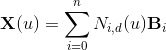
(eq. 1)

N - basis functions B - control points d - degree u - input parameter The degree of the curve d is a natural number that must be so that 1 <= d <= n. Degree + 1 is equal to a number of control points influencing the shape of a curve segment. Meaning if we would choose d to be 1 that number would be 2 and we would end up with linear interpolation between two control points. Experimenting with different values for d I have found that the best balance between performance and visual quality is when d=2.

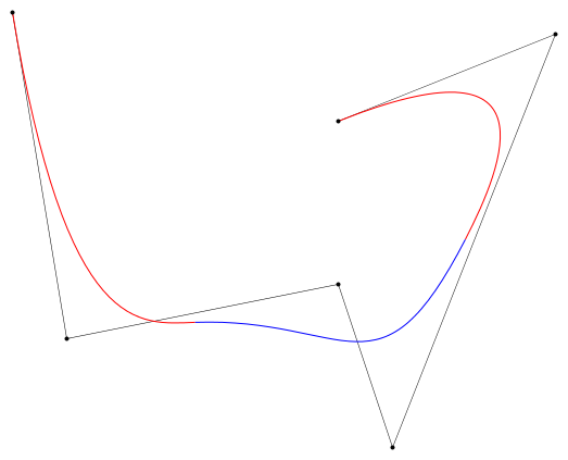Figure 1. B-spline curve

The extension from curves to surfaces is simple and is given by

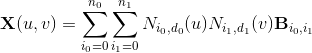
(eq. 2)

Basis function values for each, u and v parameter, are computed separately and usually stored in some array before they are used in this formula. These function values are used to determine how much every control point is influencing the end result for certain input parameter u (or u and v for surfaces). The definition for basis functions are where things get tricky.

(eq. 3)

This recursion ends when d reaches zero:

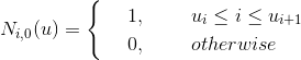
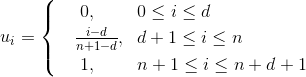
Where is a knot in a knot vector - a nondecreasing sequence of scalars. Open (nonperiodic) and uniformly spaced knot vector is used here. Also for every i. As stated before, n + 1 is the actual number of control points (according to definition), but this is inconvenient for our code. This is why, in code, the denominator is subtracted by 1. Here is the definition and code implementation:

float GetKnot(int i, int n) 
{
  // Calcuate a knot form an open uniform knot 
  vector return saturate((float)(i - D) / (float)(n - D)); 
} 

This recursive dependencies can be put into table and it can easily be seen that for a given u only one basis function N in the bottom row is not zero.

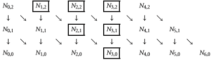
Figure 2. Recursive dependencies of a basis functions (n=4, d=2). For a certain u the only non zero values are in the rectangles.

This is the motivation behind De Boor's algorithm which optimizes the one based on mathematical definition. Further optimization is also possible like the one from the book by David H. Eberly. I have modified David's algorithm slightly so that it can run on the GPU and added some code for normal and tangent computation. So how do we get the right i so that for given u? Well considering that knot vector is uniformly spaced it can be easily calculated. One thing to note though, since u when u=1 we will end up with incorrect values. This can be fixed by making sure a vertex with a texture coordinate (either u or v) equal to 1 is never processed, which is inconvenient. The simpler way is used here, as we simply multiply the u parameter by a number that is "almost" 1.

int GetKey(float u, int n) 
{
	return D + (int)floor((n - D) * u*0.9999f);
} 

The last thing we need before any of this code will work is our constant buffer and pre-processor definitions. Although control points array is allocated to its maximum size, smaller sizes are possible by passing values to gNU and gNV. Variable gCenter will be discussed later, but besides that all variables should be familiar by now.

#define MAX_N 10 // maximum number of control points in either direction (U or V) 
#define D 2 // degree of the curve 
#define EPSILON 0.00002f // used for normal and tangent calculation 

cbuffer cbPerObject 
{ 
	// B-Spline 
	int gNU; // gNU actual number of control points in U direction 
	int gNV; // gNV actual number of control points in V direction 
	float4 gCP[MAX_N * MAX_N]; // control points 
	float3 gCenter; // arithmetic mean of control points 
	
	// ... other variables 
}; 

The function tasked with computing B-spline inputs just texture coordinates (u and v) and uses it to compute position, normal and tangent. We will add the Coordinates u and v a small epsilon value to produce an offset in coordinate space. These new values are named u_pdu and v_pdv in code and here is how they are used to produce tangent and normal:

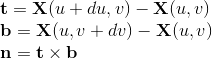
(eq. 4)

Now, as mentioned earlier, basis function values are computed and stored in separate arrays for u and v parameter, but since we have additional two parameters u_pdu and v_pdv a total of four basis functions (arrays) will be needed. These are named basisU, basisV, basisU_pdu, basisV_pdv in code. GetKey() function is also used here to calculate the i so that for given u as stated before and separately one i for given v. One might think that we also need separate i for u_pdu and v_pdv. That would be correct according to definition, but the inaccuracy we get from u_pdu and v_pdv potentially not having the correct i and thus having inacurate basis function values array is too small to take into account.

void ComputePosNormalTangent(in float2 texCoord, out float3 pos, out float3 normal, out float3 tan) 
{
	float u = texCoord.x;
	float v = texCoord.y;
	float u_pdu = texCoord.x + EPSILON;
	float v_pdv = texCoord.y + EPSILON;
	int iU = GetKey(u, gNU);
	int iV = GetKey(v, gNV); // create and set basis 
	float basisU[D + 1][MAX_N + D];
	float basisV[D + 1][MAX_N + D];
	float basisU_pdu[D + 1][MAX_N + D];
	float basisV_pdv[D + 1][MAX_N + D];
	basisU[0][iU] = basisV[0][iV] = basisU_pdu[0][iU] = basisV_pdv[0][iV] = 1.0f; 

// ... the rest of the function code 

Now for the actual basis function computation. If you look at figure 2. you can see that non zero values form a triangle. Values of the left diagonal and right vertical edge are computed first since each value depends only on one previous value. The interior values are then computed using eq. 3. Every remaining value of the basis functions array is simply left untouched. Their value is zero but even if it would be some unwanted value it doesn't matter as will be seen later.

// ... the rest of the function code 
// evaluate triangle edges [unroll] 
for (int j = 1; j <= D; ++j) 
{
  float gKI; 
  float gKI1;
  float gKIJ;
  float gKIJ1; // U 
  
  gKI = GetKnot(iU, gNU);
  gKI1 = GetKnot(iU + 1, gNU);
  gKIJ = GetKnot(iU + j, gNU);
  gKIJ1 = GetKnot(iU - j + 1, gNU);
  float c0U = (u - gKI) / (gKIJ - gKI);
  float c1U = (gKI1 - u) / (gKI1 - gKIJ1);
  basisU[j][iU] = c0U * basisU[j - 1][iU];
  basisU[j][iU - j] = c1U * basisU[j - 1][iU - j + 1];
  float c0U_pdu = (u_pdu - gKI) / (gKIJ - gKI);
  float c1U_pdu = (gKI1 - u_pdu) / (gKI1 - gKIJ1);
  basisU_pdu[j][iU] = c0U_pdu * basisU_pdu[j - 1][iU];
  basisU_pdu[j][iU - j] = c1U_pdu * basisU_pdu[j - 1][iU - j + 1]; // V
  
  gKI = GetKnot(iV, gNV);
  gKI1 = GetKnot(iV + 1, gNV);
  gKIJ = GetKnot(iV + j, gNV);
  gKIJ1 = GetKnot(iV - j + 1, gNV);
  float c0V = (v - gKI) / (gKIJ - gKI);
  float c1V = (gKI1 - v) / (gKI1 - gKIJ1);
  basisV[j][iV] = c0V * basisV[j - 1][iV];
  basisV[j][iV - j] = c1V * basisV[j - 1][iV - j + 1];
  float c0V_pdv = (v_pdv - gKI) / (gKIJ - gKI);
  float c1V_pdv = (gKI1 - v_pdv) / (gKI1 - gKIJ1);
  basisV_pdv[j][iV] = c0V_pdv * basisV_pdv[j - 1][iV];
  basisV_pdv[j][iV - j] = c1V_pdv * basisV_pdv[j - 1][iV - j + 1];
} 

// evaluate triangle interior [unroll] 
for (j = 2; j <= D; ++j) 
{ 
  // U [unroll(j - 1)] 
  for (int k = iU - j + 1; k < iU; ++k) 
  {
    float gKK = GetKnot(k, gNU);
    float gKK1 = GetKnot(k + 1, gNU);
    float gKKJ = GetKnot(k + j, gNU);
    float gKKJ1 = GetKnot(k + j + 1, gNU);
    float c0U = (u - gKK) / (gKKJ - gKK);
    float c1U = (gKKJ1 - u) / (gKKJ1 - gKK1);
    basisU[j][k] = c0U * basisU[j - 1][k] + c1U * basisU[j - 1][k + 1];
    float c0U_pdu = (u_pdu - gKK) / (gKKJ - gKK);
    float c1U_pdu = (gKKJ1 - u_pdu) / (gKKJ1 - gKK1);
    basisU_pdu[j][k] = c0U_pdu * basisU_pdu[j - 1][k] + c1U_pdu * basisU_pdu[j - 1][k + 1];
  } 
  
  // V [unroll(j - 1)] 
  for (k = iV - j + 1; k < iV; ++k)
  {
    float gKK = GetKnot(k, gNV);
    float gKK1 = GetKnot(k + 1, gNV);
    float gKKJ = GetKnot(k + j, gNV);
    float gKKJ1 = GetKnot(k + j + 1, gNV);
    float c0V = (v - gKK) / (gKKJ - gKK);
    float c1V = (gKKJ1 - v) / (gKKJ1 - gKK1);
    basisV[j][k] = c0V * basisV[j - 1][k] + c1V * basisV[j - 1][k + 1];
    float c0V_pdv = (v_pdv - gKK) / (gKKJ - gKK);
    float c1V_pdv = (gKKJ1 - v_pdv) / (gKKJ1 - gKK1);
    basisV_pdv[j][k] = c0V_pdv * basisV_pdv[j - 1][k] + c1V_pdv * basisV_pdv[j - 1][k + 1];
  }
} // ... the rest of the function code 

And finally, with basis function values computed and saved in arrays we are finally ready to use eq. 1. But before that there is one particular thing that should be discussed here. If you know how float numbers work (IEEE 754) then you know that if you add a very small number (like our EPSILON) and a very big one you could end up losing data. This is exactly what happens if control points are relatively far from world's coordinate system origin and vectors like pos_pdu and pos that should be different by a small amount end up being equal. To prevent this all control points are translated more towards center with the gCenter variable. This variable is a simple arithmetic mean of all the control points.

  // ... the rest of the function code 
  float3 pos_pdu, pos_pdv;
  pos.x = pos_pdu.x = pos_pdv.x = 0.0f;
  pos.y = pos_pdu.y = pos_pdv.y = 0.0f;
  pos.z = pos_pdu.z = pos_pdv.z = 0.0f;

  // [unroll(D + 1)] 
  for (int jU = iU - D; jU <= iU; ++jU) 
  {
    // [unroll(D + 1)]
    for (int jV = iV - D; jV <= iV; ++jV)
    {
      pos += basisU[D][jU] * basisV[D][jV] * (gCP[jU + jV * gNU].xyz - gCenter);
      pos_pdu += basisU_pdu[D][jU] * basisV[D][jV] * (gCP[jU + jV * gNU].xyz - gCenter);
      pos_pdv += basisU[D][jU] * basisV_pdv[D][jV] * (gCP[jU + jV * gNU].xyz - gCenter);
    }
  }

  tan = normalize(pos_pdu - pos);
  float3 bTan = normalize(pos_pdv - pos);
  normal = normalize(cross(tan, bTan));
  pos += gCenter;
} 

Hardware tessellation and geometry shader

Still with me? Awesome, since it is mostly downhill from this point. It was probably easy to guess that a mesh in form of a grid will be needed here, made so that its texture coordinates stretch from 0 to 1. An algorithm for this should be easy to implement and I will leave it out. It is useless to have position values of vertices in the vertex structure since that data is passed through control points (gCP). This is what vertex input structure and vertex shader needs to be like:

struct V_TexCoord { float2 TexCoord : TEXCOORD; }; 
V_TexCoord VS(V_TexCoord vin) 
{
  // Just a pass through shader 
  V_TexCoord vout; 
  vout.TexCoord = vin.TexCoord;
  return vout;
} 

The tessellation stages start with a hull shader. Tessellation factors are calculated in constant hull shader ConstantHS() while control hull shader HS() is again, like VS(), a passthrough shader. Although at first I experimented and created per-triangle tessellation, it was cleaner, faster and easier to implement per-object tessellation, so that approach is presented here.

struct PatchTess 
{
  float EdgeTess[3] : SV_TessFactor;
  float InsideTess : SV_InsideTessFactor;
};

PatchTess ConstantHS(InputPatch patch, uint patchID : SV_PrimitiveID)
{ 
  PatchTess pt; // Uniformly tessellate the patch. 
  float tess = CalcTessFactor(gCenter);
  pt.EdgeTess[0] = tess;
  pt.EdgeTess[1] = tess;
  pt.EdgeTess[2] = tess;
  pt.InsideTess = tess;
  return pt;
}

[domain("tri")] 
[partitioning("fractional_odd")]
[outputtopology("triangle_cw")]
[outputcontrolpoints(3)]
[patchconstantfunc("ConstantHS")]
[maxtessfactor(64.0f)]

V_TexCoord HS(InputPatch p, uint i : SV_OutputControlPointID, uint patchId : SV_PrimitiveID) 
{ 
  // Just a pass through shader 
  V_TexCoord hout; 
  hout.TexCoord = p.TexCoord;
  return hout;
} 

Also a method for calculating tessellation and a supplement for our constant buffer cbPerObject. Since control points are already in world space, only view and projection matrices are needed and here they are supplied already multiplied as gViewProj. Variable gEyePosW is a simple camera position vector and all variables under the "Tessellation" comment should be self-explanatory. CalcTessFactor() gets us the required tessellation factor used in HS() by a distance based function. You can alter the way this factor changes with distance by setting different exponents of the base s.

cbuffer cbPerObject 
{ 
  // ... other variables
  // Camera 
  float4x4 gViewProj; 
  float3 gEyePosW; 
  
  // Tessellation 
  float gMaxTessDistance;
  float gMinTessDistance;
  float gMinTessFactor;
  float gMaxTessFactor;
};

float CalcTessFactor(float3 p) 
{
  float d = distance(p, gEyePosW);
  float s = saturate((d - gMinTessDistance) / (gMaxTessDistance - gMinTessDistance));
  return lerp(gMinTessFactor, gMaxTessFactor, pow(s, 1.5f));
} 

Now in domain shader we get to use all that B-spline goodness. New structure is also given, as here we introduce position, normals and tangents. Barycentric interpolation is used to acquire the texture coordinates from a generated vertex and then used as u and v parameters for our ComputePosNormalTangent() function.

struct V_PosW_NormalW_TanW_TexCoord 
{
  float3 PosW : POSTION;
  float3 NormalW : NORMAL;
  float3 TanW : TANGENT;
  float2 TexCoord : TEXCOORD;
};

[domain("tri")]
V_PosW_NormalW_TanW_TexCoord DS(PatchTess patchTess, float3 bary : SV_DomainLocation, const OutputPatch tri) 
{
  float2 texCoord = bary.x*tri[0].TexCoord + bary.y*tri[1].TexCoord + bary.z*tri[2].TexCoord;
  V_PosW_NormalW_TanW_TexCoord dout;
  ComputePosNormalTangent(texCoord, dout.PosW, dout.NormalW, dout.TanW);
  dout.TexCoord = texCoord;
  return dout;
} 

And now the final part before passing vertex data to pixel shader. The geometry shader. Why? Well because cloth is visible from both sides, DUH! Triangles in DirectX graphics pipeline are not however and even if we disable backface culling, the normals would still have opposite values on the back face of a triangle. This is where GS() comes in. We input three vertices at once from DS() (one triangle) and copy them to the output stream. Additionally, three more vertices are added with only difference in normal. Another thing worth mentioning is that PosW is transformed to homogeneous clip space (projection space) and saved to PosH. This is the reason for this new structure:

struct V_PosH_NormalW_TanW_TexCoord 
{
  float4 PosH : SV_POSITION;
  float3 NormalW : NORMAL;
  float3 TanW : TANGENT;
  float2 TexCoord : TEXCOORD;
};

[maxvertexcount(6)]
void GS(triangle V_PosW_NormalW_TanW_TexCoord gin[3], inout TriangleStream triStream) 
{
  V_PosH_NormalW_TanW_TexCoord gout[6];
  
  [unroll] // just copy pasti'n 
  for (int i = 0; i < 3; ++i) 
  {
    float3 posW = gin.PosW;
    gout.PosH = mul(float4(posW, 1.0f), gViewProj);
    gout.NormalW = gin.NormalW;
    gout.TanW = gin.TanW;
    gout.TexCoord = gin.TexCoord;
  }
  
  [unroll] // create the other side 
  for (i = 3; i < 6; ++i) 
  {
    float3 posW = gin[i-3].PosW;
    gout.PosH = mul(float4(posW, 1.0f), gViewProj);
    gout.NormalW = -gin[i-3].NormalW;
    gout.TanW = gin[i-3].TanW;
    gout.TexCoord = gin[i-3].TexCoord;
  }
  
  triStream.Append(gout[0]);
  triStream.Append(gout[1]);
  triStream.Append(gout[2]);
  triStream.RestartStrip();
  triStream.Append(gout[3]);
  triStream.Append(gout[5]);
  triStream.Append(gout[4]);
} 

I will leave it to the reader to decide what to do in pixel shader. With normals, tangents and texture coordinates there should be everything needed to create all kinds of visual magic. Good luck!

float4 PS(V_PosH_NormalW_TanW_TexCoord pin) : SV_Target 
{
  // ... now what?! XD 
}

technique11 BSplineDraw 
{
  pass P0 
  {
    SetVertexShader(CompileShader(vs_5_0, VS()));
    SetHullShader(CompileShader(hs_5_0, HS()));
    SetDomainShader(CompileShader(ds_5_0, DS()));
    SetGeometryShader(CompileShader(gs_5_0, GS()));
    SetPixelShader(CompileShader(ps_5_0, PS()));
  }
} 

Conclusion

Although this is not a complete shader and the work being done on the CPU is not covered at all, I think this article will give a good start to anybody wanting to have fast and pleasant looking cloth simulation in their engines. Here is a file that contains all the written code in orderly fashion and should be free from bugs and errors. Also, you can follow me on Twitter and check out this

 which demonstrates explained methods in action. Hope you like it!