Notes about this article series
This is the first article in a series dedicated to realistic natural phenomena rendering. Starting with water, each natural effect will be extensively covered by 3 to 5 individual articles. It is not meant to be a tutorial, nor an academic paper, but a comprehensive and in depth guide for the intermediate to experienced graphics programmer. Each effect is covered from the basic aspects to the more advanced details, and various implementation approaches are discussed. The series focuses mainly on the practical aspects of nature effect implementation. Source snippets and pseudo code are provided for many important functions, and the amount of math is kept to the relevant minimum.
The series tries to be as platform agnostic as possible, concrete examples are however written according to the OpenGL API. This has a few implications for users of other APIs: all matrices are column major order, texture coordinates are named s, t, r and q, and are assumed in the 0 to 1 range. All matrices are assumed to be 4x4 unless otherwise stated. Many of the effects presented are very shader heavy, mostly targeting current generation 3D chipsets. All shader code is written in the API independent Cg language [1], porting it to a different high level shader language (such as GLSL or HLSL) should be straightforward.
Introduction
CG water has been a major research topic for a long time now. Realistically simulating liquids has proven very difficult, due to the inherent complexity of the physical processes involved. Most photorealistic solutions use a form of raytracing and complex differential equations to approximate the optical behaviour and motion dynamics of a water body. Unfortunately, such physically accurate approaches often take many hours of render time per frame. With the advance of programmable 3D hardware, many algorithms previously limited to offline processing have become available for realtime usage. But as always when implementing complex effects in interactive contexts such as video games, quality versus performance tradeoffs must be made. A lot of the visual properties of water can be approximated by efficient techniques that, even though not physically correct, look convincing to the human eye.
This water series will discuss many such techniques, focussing on the simulation of finite size constrained water bodies. Both dynamic and optical properties will be covered. The basic water simulation targets ps1.3 / fp20 compliant 3D chipsets, the more advanced effects requires a ps2.0 / arbfp1 capable GPU.
Simulating water
As most physically based effects, water simulation is a combination of two distinct steps. The physical generation step, often called the wave model, simulates the motion of a water body under the influence of many different internal and external forces. The wave model is what makes the water move, change shape, and interact with its environment. Mathematically, many different approaches are possible. The simple ones apply procedural noise, often in the form of Perlin noise [2], simulating a rough and seemingly random movement without much user interaction. The more realistic ones often try to mimic the motion of a real water body by solving differential equations, approximating the physical laws of hydrostatics and hydrodynamics, and offering full interactivity between the player and the water.
The second step is the visualization, which takes the water data computed by the wave model, and renders it onto the screen. For high realism, physical laws need to be taken into account again. A water surface exhibits complex interactions with the light from the environment, modelling these optical properties is crucial for a visually compelling result. Unlike the wave model, which can be computed on the CPU, the optical simulation of the water surface often requires complex terms to be evaluated per pixel. Modern ps2.0 level 3D hardware, offering both per-vertex and per-pixel programmability, is perfectly suited for this task.
Finding a water representation
The wave model passes the information to the water renderer through a common data interface. Using a simple and abstract representation of the water body offers the advantage of high modularity: different wave models and renderers can access the same data set without requiring conversion and knowledge of each other. This is an important feature when adding both physical and visual level of detail schemes later on. Selecting an appropriate intermediate representation is an important aspect of water generation, and will impact on performance and visual quality of the simulation.
The most natural representation of a liquid such as water is conceptually a particle system. While a simulation on molecular level is still impossible for obvious reasons, the approach can be made practical on a coarser level, by increasing the particle size. Each particle carries state information about a small subset of the water body, and is subject to a multitude of external forces acting on it. The particle state, such as velocity and position within the volume, as well as possible collision situations are resolved and updated by the wave model. The rendering is often done via meta particles, usually by an isosurface generation technique such as the well known marching cubes algorithm.
Such a particle based approach offers the advantage of a very realistic and flexible framework, which doesn't impose any spatial constraints onto the water body. While realtime implementations are possible on a reduced number of particles, practical usage in games is limited due to the very high performance requirements. An alternative approach would therefore be desirable. The most performance intensive part of the particle model is the tracking of interactions between individual particles, and collisions with the outer environment. This step can be largely simplified by making the particle positions invariant - essentially replacing them by a fixed grid voxel field. Instead of tracking the trajectory of each individual particle through the water body, the voxel approach tracks the physical state of the liquid as it changes over a grid of fixed cells.
The main advantage of a voxel representation is computational speed and implementation simplicity. Due to the nature of the fixed grid structure, interactions between adjacent cells can be efficiently computed. The precision of the simulation is given by the grid resolution, offering good hardware scalability and the possibility of speed vs. accuracy tradeoffs. A water body approximated by a 3D voxel grid offers much of the flexibility a more general particle model would provide, at a considerably lower performance impact. However, the voxel technique also suffers from inherent limitations. A particle-based system is open; it can operate within a virtually infinite spatial domain. A voxel based simulation is restricted to the spatial extends covered by the voxel field, and is therefore a closed system. As long as the liquid is kept within the boundaries of this system, might it be by forces such as gravity or by external geometric limits (boundary conditions), the results will be comparable to a particle system constrained by the same external conditions. But as soon as liquid exits the closed system, its state becomes undefined, as it isn't covered by the voxel representation anymore. A possible solution is to expand the field as necessary, either by increasing the distance between cells (losing precision, but keeping computational cost constant), or by adding cells at the appropriate side(s) of the field (keeping precision, but increasing the computational overhead). The best solution is to avoid such expansion altogether, by providing adequate physical constraints to the liquid (for example keeping water in a closed container such as a glass or a pool).
Although being more efficient than large particle systems, solving and rendering 3D voxel based water can still become prohibitively expensive with increasing resolution of the grid. Especially in the context of a video game, where high frame rates are required, yet only a small fraction of the available frame time can be dedicated to water simulation, maximal speed is essential.
An important observation is that typical 3D games rarely require a full 3D simulation of large water volumes. In fact, volumetric water is often limited to small and highly localized effects, such as for example a running water tap, or a waterfall. These effects can often be approximated by standard particle systems, and won't benefit from a complex physically based solution. In many cases, the water effects with the largest visual impact are not defined by their full volumetric behaviour, but by the appearance of the surface: from water puddles, over smaller pools and submerged areas, to entire lakes or oceans. All those water bodies have in common, that the precise dynamics below their surface are of secondary importance, often even completely invisible to the player. Their visual aspect is almost entirely defined by the dynamic properties of their surface. Ripples, waves, turbulences, along with the optical interactions they create are what make water look realistic.
Unfortunately, the 3rd dimension cannot simply be dropped completely in favour of a purely 2D surface model. Volume has to be taken into account while computing the surface dynamics. The best way to combine both worlds is by using a 2.5D representation, commonly known as a heightfield. Each 2D grid cell stores the height of the water from the bottom (which is assumed flat) to the surface at position [x, y]. This extrusion defines a volume of water for each column, V = dx * dy * height, where dx is the size of a grid cell in horizontal direction, dy the size in vertical direction, and height the value stored in the cell at [x, y]. This trick allows the physical wave model to operate on a 3D water volume, while restricting all calculations to a single 2D slice of the volume data set: the surface.
A heightfield offers several advantages beyond fast 2D calculations, such as easy rendering and low memory consumption. Converting a heightfield to a geometric mesh is very straightforward as no complex isosurface generation is required. Heightfields have been extensively researched for terrain rendering, most of the LOD and VSD techniques developed for terrains can be directly applied to water heightfields. Of course, water heightfields also inherit a set of limitations from their terrain counterparts: they're essentially extruded 2D maps, and can only simulate a subset of the physical effects a full 3D voxel field can. The slope of the mesh connecting two adjacent cells is limited to angles below 90°, which restricts the model to individually convex waves (i.e. no breaking waves). Also, only water under the influence of gravity can be simulated by a planar heightfield, zero gravity water requires a full 3D grid. In practice however, usability rarely suffers from those drawbacks, and the advantage of high performance outweighs the limitations.
Optical properties of real life water
The next sections assume that a valid water surface heightfield, along with the grid normals is available, and will discuss the visual properties of the surface needed for realistic rendering. Several different wave models and methods of heightfield generation will be discussed later in this series.
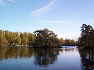
When looking closer at the movement of a water surface, it becomes apparent that dynamics are distributed over the entire frequency spectrum. From large scale, low frequency features such as long and slow waves, to very small high frequency turbulences that almost seem chaotic and unpredictable in nature. Water is in fact a multi-resolution phenomenon, and this large dynamic range of possible fluctuations needs to be taken into account in order to achieve a realistic result under all viewing conditions. Fast vertex processing can conveniently approximate large-scale features, while small scale turbulences have to be treated per pixel.The final goal being the photorealistic rendering of a water surface, one should start by examining the visual properties of real world water. Consider the picture of a calm lake (Fig. 1). The first optical effect that strikes the eye is the reflection of the environment in the water. Incoming light from the environment is reflected by the surface, which essentially acts like a large mirror.
This reflection is not perfectly stable and clear, but distorted by the turbulences of the surface. Next, when looking down through the water body to the ground, an effect known as refraction becomes apparent. When light passes through the boundary between two media of different density, it changes its direction due to the light speed differential. In this specific case, one medium is air, the other one is the water, and the boundary is the surface. From a visual point of view, refraction distorts the image of all objects under water, again according to the dynamics of the surface. Now, it seems light can sometimes be reflected by the surface and sometimes be transmitted through the water body. The ratio of reflected versus transmitted light at a certain point on the surface is determined by several factors. The most important one is the angle of the viewer to the surface. Consider again a real life lake. When looking straight down into the water, at a very large view angle, the surface is almost fully transparent and no reflection takes place. However, when looking at the surface from a distance, the view angle becomes smaller and the amount of reflection increases. At the same time, the transparency decreases, until the water surface becomes almost completely opaque. This optical property is called the Fresnel effect.
Until now, perfectly clear and fully transparent water was assumed. In reality, water almost always contains a varying amount of impurities, most often in the form of small dirt particles floating in suspension. These particles, as well as the water molecules themselves, alter the optical properties by scattering and absorbing part of the transmitted light, decreasing the visibility under water and creating effects such as light shafts. They are the reason why shallow water seems more transparent than deep water. The longer the distance light has to travel through the medium, the higher the probability for it to be scattered or absorbed by a particle or molecule. Besides its effect on translucency, wavelength dependent light scattering and absorption gives water its inherent colouring, such as the commonly encountered blue and greenish tones.
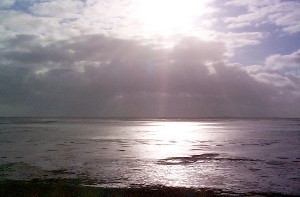
Last but not least, water is an excellent specular reflector at shallow angles. The specular part of the standard Phong lighting model can be applied to the surface, using a large specular exponent. Fig. 2 shows the typical light band resulting from specular reflection. Under certain view angles, water can almost act as a perfect mirror, reflecting incoming light directly towards the viewer. Under high intensity light, such as from the sun, those direct reflected light paths result in bright sparkles (Fig. 3)
Rendering reflections with cubemaps
Since the introduction of hardware support for cubemaps, cubic environment mapping became a popular method of rendering reflective geometry [3]. Incident light around a specific point in space is stored in the environment map, which acts as a 360° lookup table. The cubemap is indexed by a 3-component direction vector, and returns the incoming light from the direction pointed by the vector. This behaviour can be used to create reflective objects. First, an RGBA image of the environment is stored in the cubemap: a camera with a 90° FOV is positioned at the centre of the cubemap, and six images are rendered along the major axes onto the respective sides of the cube. The environment, as seen over a full 360° sphere around the centre point is now encoded in the map. This step can be precomputed, if the environment is static. In a second pass, the reflective object is rendered, and a reflection vector is computed at each vertex or pixel. This reflection vector is used as an index into the environment cubemap, essentially retrieving the incoming light from the direction of the reflected view ray. Source 1 shows a simple vertex and pixel shader performing reflection using the cubemap approach (vertices and cubemap are assumed to be in world space).
void VP_cube_reflect( float4 inPos : POSITION,
                      float3 inNormal : NORMAL,
                      out float4 outPos : POSITION,
                      out float3 outTexCube : TEXCOORD0,
                      uniform float4x4 Mvp,
                      uniform float3 cameraPos )
{
    // transform vertex position by combined view projection matrix
    outPos = mul(Mvp, inPos);

    // create ray from camera position to the vertex, in world space
    float3 V = inPos - cameraPos;

    // compute the reflection vector, and assign it to texcoord 0
    outTexCube = reflect(V, inNormal);
}

void FP_cube_reflect( float3 inTexCube : TEXCOORD0,
                      out float4 outCol : COLOR,
                      uniform samplerCUBE EnvCubeMap )
{
    // sample cubemap with the reflection vector
    outCol = texCUBE(EnvCubeMap, inTexCube);
}
Source 1: cubemap reflection shader
However, environment mapping suffers from a critical drawback. Since the incoming light is only sampled around a single point in space, it is only valid for an object, if the environment is assumed to be infinitely far away. While this assumption usually holds up pretty well for very large distance environments such as sky scapes (for example the well known skybox), local reflections cannot be represented at all. The attempt of refleting a local object using an environment cubemap with result in severe visual artifacts. Still, the algorithm has the advantage of being single pass with static skies, making it a very fast method of adding reflections onto water surfaces without direct local geometry. It can also handle very steep waves, making it optimal for rough water bodies such as the ocean.
Tip:
Under certain circumstances, the reflection vector can point downwards, into the lower hemisphere of the cubemap. In reality, this leads to the water reflecting itself (often recursively), which we cannot model directly. A way to fake the visual appearance of such interreflections is to first mirror the upper half of the cubemap down into the lower half, then tint the lower half using the general water colour, and finally run it through a Gaussian blur filter. When using a static environment, this process can be precomputed offline and stored with the cubemap.
Planar mirrors for local reflections
The largest problem with cube environment mapping is the lack of local reflections. An interesting alternative is the planar mirror technique, also known under the slight misnomer "stencil reflection". Often used as general-purpose reflection algorithm on flat opaque geometry, such as for example shiny marble or glass, it is perfectly able to handle both local and distant reflections. Although the approach will only work on totally planar reflectors, a water surface is usually flat enough to be approximated by a single reflective plane. The results won't be physically accurate, but the visual appearance is very convincing. Planar mirrors are easy to implement, and existing engine functionality can often be reused. The effect is view dependent, and consists of two main passes that have to be executed once per frame.
On the first pass, the environment is geometrically reflected around the water plane by the use of a special reflection matrix. Assume a coordinate system with X and Y parallel to the ground, and positive Z upwards. Since an undisturbed water surface under the influence of gravity will always be parallel to the ground, the plane approximating the surface will always have a constant surface normal of [0, 0, 1]. The reflection operation is therefore reduced to a geometric scale of (-1) on the Z axis (essentially flipping it around), but additional care must be taken if the water plane does not cross the origin. Given the height h of the water surface from the ground, the final reflection matrix Mf is shown below:
1 0 0 0
0 1 0 0
0 0 -1 2h
0 0 0 1
The environment reflected through Mf is then rendered from the point of view of the original camera into a 2D reflection texture. Note that the common stencil based reflection technique cannot be applied to water reflections, the image needs to be available as a texture. Caveat: the above reflection matrix assumes vertex coordinates to be in world space. Where this is not the case, the local object transformation matrix (Mo) needs to be applied first. The typical concatenated view matrix used to render a reflected environment is as follows, where Mc is the current camera matrix, and Mreflview the final reflected view matrix:
Mreflview = Mc * Mf (* Mo)
Tip:
Since the geometric reflection is essentially a negative scale, the winding order of the primitives rendered with the reflection matrix enabled will be inverted. This can lead to visual anomalies if backface culling and/or two-sided lighting is enabled. The solution is to either flip the backface culling mode from front to back (or vice-versa), or to invert the internal winding order of the 3D API.
In the second pass, the reflection texture is applied to the water mesh using projective texturing. The result is a perfectly calm reflection of the environment onto the water surface. Although features such as waves or turbulences distort the reflection in reality, the current model doesn't take any of this into account yet, as it has no knowledge about the dynamic state of the surface. Fortunately, projective texturing allows the manipulation of the projective coordinates either per vertex or per pixel. This can be used to realistically distort the projected reflection image according to the current water surface state.
A word on projective texturing
Planar mirrors as described above require projective texturing in the second pass. Projective texture mapping [4] is a technique where a 2D texture is projected onto an object, rather than being directly attached to it (as it would be with conventional texture mapping). It operates analogous to a slide projector, where an image, or rather its texture coordinates are projected onto an object. From the concept, it does the exact opposite of a camera: instead of recording an image of the environment by means of an orthographic or perspective projection, projective texture mapping projects an image onto the environment, by using a matrix very similar to the one a camera uses. Both perform the same operations on a vertex, the difference lies in the way the resulting coordinates are processed. The camera model uses the transformed and projected vertex positions to rasterize a primitive onto the screen, while perspective texture mapping uses them to index a texture.
General projective texture mapping allows such a "slide projector" to be positioned virtually anywhere in the scene. But the way it is used by the planar reflection technique is a special and simplified case. In fact, the projector position and orientation is exactly equal to the camera position and orientation. Both share the same view and projection matrices, which make things a lot easier. Imagine the camera being a combined recording and projecting device, that records the (reflected) environment during the first pass to a texture, and projects it back onto the water surface during the second pass (although not reflected).
The math behind projective texture mapping is pretty straightforward, and is very similar to the way vertices are processed by the standard viewing pipeline. First, the vertex position is multiplied by the view and projection matrices, transforming it to clip space. At this point, a remapping operation unique to projective texturing is performed. A clip space coordinate c has a defined range of [-1 < c < +1], in both x and y directions (the z component is handled differently depending on the API, but it can safely be ignored in the context of projective reflections). But since the transformed vertex position will be used as a texture coordinate, it has to be remapped to the 0 to 1 range required to access a texture map. This is simply done by dividing each component of the clip space position by 2, and adding 0.5 to the result. This operation can be conveniently expressed by a 4x4 remapping matrix Mr:
0.5 0 0 0.5
0 0.5 0 0.5
0 0 0.5 0.5
0 0 0 1
As mentioned above, in the case of planar mapping, the camera view matrix Mc and the camera projection matrix Mp are equivalent to the matrices used by the projective mapping step. When rendering the water surface in step 2 of the planar reflection algorithm, the projective texture coordinates used to apply the reflection texture are computed by transforming the world space water grid vertex positions by the following combined projective texture matrix Mprojtex:
Mprojtex = Mr * Mp * Mc
The resulting projective texture coordinates show a property that might seem unusual to someone used to conventional 2D [s, t] coordinate pairs: their homogeneous coordinate q is not automatically one, and can therefore not simply be ignored. This is due to the projection encoded in Mp and relates to the homogeneous w coordinate used in the standard viewing pipeline. In the same way x and y are divided by w ("homogeneous divide"), the projective texture coordinates s and t need to be divided by q. This is achieved by a special projective texture access opcode within the pixel shader, which internally uses a [s/q, t/q] pair to access the texture rather than the conventional [s, t] pair. Cg uses the tex2Dproj keyword for this purpose. Source 2 shows a basic vertex and pixel shader combo to perform projective texture mapping in the context of planar reflections.
void VP_projective( float4 inPos : POSITION,
                    out float4 outPos : POSITION,
                    out float4 outTexProj : TEXCOORD0,
                    uniform float4x4 Mvp,
                    uniform float4x4 Mprojtex )
{
   // transform vertex position by combined view projection matrix
   outPos = mul(Mvp, inPos);
   // transform vertex position by projective texture matrix and
   // copy the result into homogeneous texture coordinate set 0
   outTexProj = mul(Mprojtex, inPos);
}

void FP_projective( float4 inTexProj : TEXCOORD0, out float4
outCol : COLOR, uniform sampler2D ReflectMap )
{
   // projectively sample the 2D reflection texture
   outCol = tex2Dproj(ReflectMap, inTexProj);
}
Source 2: projective texture shader
Tip:
Mvp is the combined view projection matrix. Instead of explicitly multiplying a vertex by two distinct matrices (the camera view matrix, followed by the projection matrix), one can concatenate both matrices into the combined view-projection matrix for performance reasons. Mvp will directly transform a world space point into clip space, without going over camera space. Mathematically speaking, Mvp = Mp * Mc. If a vertex is originally in local object space instead of world space, then it first needs to be transformed to world space. In this case, Mvp = Mp * Mc * Mo holds true. This latter combined matrix is often called the modelview-projection matrix, and will map a vertex from local object space into clip space.
Clipping planes
When creating the reflection texture as described in the first step of the planar mirror algorithm, it was assumed that all reflected objects are initially above the water surface. This rarely is the case under real conditions, except perhaps for simple test scenes. There will almost always be geometry and objects below the water surface, often they will even intersect it. When reflecting the environment around the water plane, geometry that was below the surface will suddenly end up above it. These parts need to be clipped away, otherwise visual artifacts in the form of ghost reflections can appear.
Many approaches to geometric clipping exist, and all of them will achieve the desired results. But depending on the choice of target hardware and the complexity of the reflected geometry, some may be better suited than others, especially from performance considerations and feature requirements. Discussing the details of geometric clipping would be out of scope for this article, but a short overview over the most common techniques and their benefits and drawbacks when combined with water reflections is shown below:
User clip plane
User clip planes are provided as a built-in feature of many 3D APIs. They are easy to use and portable. Unfortunately, hardware support varies, and user clip planes are not guaranteed to be hardware accelerated on many current 3D chipsets. Information about user clip planes can be found in the specifications of the selected target API.
Alpha testing
Culling away fragments using the alpha test has long been the method of choice for user plane clipping. The signed distance from a vertex to the water plane is computed and passed as 1D texture coordinate into a clamped alpha texture, after appropriate remapping. The result of the texture lookup is passed on to the alpha test, which culls away all fragments on the wrong side of the plane. This technique is hardware accelerated even on older 3D chipsets. But it burns up a texture stage, and uses the output alpha, which is often unacceptable.
Pixel shader based culling
As with alpha test culling, the signed distance from the vertex to the plane is computed, and passed to a pixel shader. The shader culls away all fragments with a negative (or positive) distance using a function such as texkill. Pixel shader based culling is efficient, but requires shader capable hardware. Also, the culling functionality has to be explicitly added to every single shader that might be used by reflective geometry.
Oblique frustum clipping
A potentially optimal culling technique developed by Eric Lengyel. It maps the standard frustum near plane onto an arbitrary user defined clipping plane (the water surface in this case) by modifying the camera projection matrix. The technique is hardware accelerated by all 3D chipsets, since it operates on functionality inherently available on all 3D architectures (standard view frustum clipping). Oblique frustum culling doesn't require any additional GPU resources. The drawback is a reduced z-buffer precision on the reflected render pass. More information about the technqiue can be found under [5].
Disturbing the reflection
Until now, the reflections are completely flat and clear, a direct consequence of the planar water surface approximation. But the water surface is often not flat at all. In fact the wave model might have given the renderer a very choppy surface, with many interfering waves and turbulences. Fortunately, the projective texture pass allows full control over the way the reflection texture is applied to the water: by modifying the projective coordinates, distortions are introduced.
The perfect mirror generated by undisturbed projective coordinates assumes all water grid normals to point straight upward, parallel to the normal of the idealized flat water surface. This assumption is correct, as long as the water surface stands perfectly still, without the slightest fluctuation. As soon as the surface starts to move, the water grid normals deviate from their ideal direction. Since the mesh generated from the water heightfield cannot represent slopes larger than 90°, the normals are also bound to this limit. In the worst-case scenario, a grid normal will be parallel to the water surface, lying on the XY plane. Along with the grid position, the grid vertex normal deviation can serve as a measure of how much directional distortion is required within the reflection. Many different mathematical approaches can be used to derive the precise distortion vectors from this information. As so often in computer graphics, choosing an appropriate technique is again a tradeoff between accuracy and speed.
While not physically accurate, a simple 2D displacement along the normal can approximate the amount and direction of the reflective distortion. This technique is very efficient, and generates good-looking results on a typical water surface. Alternative and more precise methods will be discussed later in this series. In order to compute the distortion, the vertex grid positions are displaced along their respective normal, just before being fed into the projective texture matrix Mprojtex. The displacement is only carried out on the [x, y] components of the point, while the z component is kept unmodified. This displacement will adjust the generated projective texture coordinates, shifting them into the appropriate direction proportionally to the deviation of the vertex normals. No displacement takes place on an undisturbed upwards-pointing normal. The equation used is as follows:
P.x += d * N.x
P.y += d * N.y
where P is the vertex position, N the vertex normal, and d is a user adjustable factor controlling the strength of the distortions. This factor has no specific physical meaning, the optimal value depends on the geometric scale, the wave model, and personal preference. Various values for d should be tried out, until the visual result is found to be satisfactory.
The distortion pass can be conveniently inserted into the projective vertex shader, displacing the vertex coordinates just before they are multiplied with the projective texture matrix. The modified part of the vertex shader is given in source 3:
float d = 4.0;                    // the adjustable displacement factor

float4 dPos;                      // temporary variable to hold the displaced vertex position
dPos.xy = inPos.xy + d * inNormal.xy; // displace the xy components of the vertex position
dPos.z = inPos.z;                 // the original z component is kept
dPos.w = 1.0;                     // the w component is always one for a point

outTexProj = mul(Mprojtex, dPos); // transform the displaced vertex position by
                                  // the projectivetexture matrix and copy the
                                  // result into homogeneoustexture coordinate set 0
Source 3: projective reflection coordinates displacement
Putting it all together
As a reminder, the following matrices are used throughout the reflective water algorithm:
Standard camera and view matrices
Mo
Local object matrix, transforming local object space to world space
Mc
Camera matrix, transforming world space to camera space
Mp
Camera projection matrix, transforming camera space to clip space
Mvp
Combined view projection matrix, transforming world (or object) space to clip space
Special matrices
Mf
Reflection matrix, reflects a world space object around a world space plane
Mr
Projective remapping matrix, remaps projected coordinates from clip space to texture space
Combined reflective and projective matrices
Mreflview
The reflective view matrix, transforms world (or object) space into reflected camera space
Mprojtex
The projective texture matrix, transforms world space into projective texture space
The reflective water is generated in two passes: first the environment around the water surface is reflected into a texture, and then the water mesh is rendered projecting the distorted reflection texture onto its surface:
Pass 1: reflection texture generation
- Bind a render texture as current render target: this will be the future reflection texture
- Load Mp as the current projection matrix
- Mreflview = Mc * Mf (* Mo)
- Push the model view matrix, load Mreflview as the current modelview matrix
- Enable a user clip plane at the water surface
- Invert the primitive culling / winding order
- Render the entire scene (except the water) to the currently bound render texture
- Restore the culling / winding order
- Disable user clip plane
- Pop the previous model view matrix
- Bind the framebuffer as render target
At this point, the normal 3D scene can be rendered as usual. The reflection has been saved in the reflection texture for later processing. Pass 2 will be run as soon as the engine decides to render the water surface:
Pass 2: rendering the reflective water surface
- Bind the reflection texture onto texture unit 0
- Enable the projective water vertex and fragment shaders (Listing 5)
- Mvp = Mp * Mc (* Mo)
- Mprojtex = Mr * Mp * Mc
- Bind Mvp and Mprojtex to the vertex shader
- Optionally enable alpha blending for transparent water
- Render the water grid mesh, supplying vertex positions and vertex normals
- Disable alpha blending, if applicable
- Disable both shaders
Only pass 2 requires special shaders in order to render the water surface: a vertex shader to create the distorted projective texture coordinates, and a fragment shader to perform the projective texture lookup. Alpha blending can be used to make the water surface slightly transparent. In this case, additional functionality has to be added to the shaders, in order to pass the transparency into the alpha component of the output colour. A simple example of such a basic water shader combo is given below:
void VP_water_1( float4 inPos : POSITION,
                 float3 inNormal : NORMAL,
                 out float4 outPos : POSITION,
                 out float4 outTexProj : TEXCOORD0,
                 uniform float4x4 Mvp,
                 uniform float4x4 Mprojtex )
{
   // transform vertex position by combined view projection matrix
   outPos = mul(Mvp, inPos);

   // the adjustable displacement factor
   float d = 4.0;

   // temporary variable to hold the displaced vertex position
   float4 dPos;
   // displace the xy components of the vertex position
   dPos.xy = inPos.xy + d * inNormal.xy;
   // the original z component is kept
   dPos.z = inPos.z;
   // the w component is always one for a point
   dPos.w = 1.0;

   // transform the displaced vertex position by the projective
   // texture matrix and copy the result into homogeneous
   // texture coordinate set 0
   outTexProj = mul(Mprojtex, dPos);
}

void FP_water_1( float4 inTexProj : TEXCOORD0,
                 out float4 outCol : COLOR,
                 uniform sampler2D ReflectMap )
{
   // projectively sample the 2D reflection texture
   outCol.rgb = tex2Dproj(ReflectMap, inTexProj).rgb;
   // optionally set alpha component to transparency,
   // a constant value in this simple example
   outCol.a = 0.8;
}
Source 4: projective displaced reflective water shader
The planar reflection technique described in this article allows basic water surfaces to reflect their local environment according to the surface dynamics. The next article will describe how to add refractions and account for the Fresnel effect. It will also discuss depth dependent visibility limitation, adding small-scale perpixel turbulences onto the surface, and how to perform basic specular water lighting.
References
[1] nVidia: Cg downloads
[2] Ken Perlin: Improved Noise reference implementation
[3] nVidia: Cube Map tutorial
[4] nVidia paper: Projective texture mapping
[5] Eric Lengyel, Terathon Software: Oblique frustum clipping
Copyright © 2004 by Yann Lombard. All rights reserved.
Images: http://www.freeimages.co.uk

