Abstract
Shadow generation in 3D scenes is an active area of research. Shadows provide an increased realism and give the viewer additional information about the spatial relationships in the scene and relative depth. Shadow maps provide a relatively simple approach to shadow generation and take advantage of graphics hardware to perform the calculations. Unfortunately, shadow maps suffer from an aliasing problem that makes them unsuitable for certain situations. This paper discusses techniques that have been developed over the past few years that attempt to limit the aliasing problem.
Introduction
The shadow map algorithm is a well known method for generating shadows in 3D scenes. Aliasing associated with shadow maps is also well known. This paper focuses on several types of algorithms developed in the past few years that attempt to remove some of the aliasing: perspective shadow maps [Stamminger and Drettakis 2002], scene optimized shadow maps [Chong and Gortler 2006], logarithmic shadow maps, and non-uniform rasterization [Johnson et al. 2004] [Aila and Laine 2004].
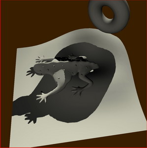
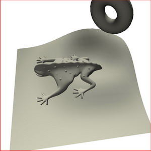
Figure 1: A scene rendered with and without shadows.
Shadow Map Algorithm
Shadow casting can be thought of as a visibility problem. Everything that is visible from the position of the light will be lit. The shadow map algorithm takes advantage of graphics hardware to perform the visibility test. To determine lighting with shadow maps requires two steps. First, the shadow map is created by rendering the scene from the point of view of the light and storing the depth value of visible geometry instead of color information. The depth information can then be accessed as a texture. Next, render the scene from the point of view of the camera. To determine if a point is in shadow, transform the point with the same transform used when creating the shadow map. The x and y coordinates correspond to the screen space coordinates and can be translated into texture coordinates for the shadow map. Finally, compare the distance from the point to the light and the value stored in the shadow map. If the distance to the light is greater than that stored in the shadow map, the point is in shadow.
Aliasing in Shadow Maps
Unfortunately, shadow maps store discreet samples of the scene. Just as there is aliasing in any 3D output, there is aliasing in the shadow map. The aliasing can cause jagged shadow boundaries. Also, a large part of the visible geometry may map back to a small part of the shadow map which exaggerates the aliasing.
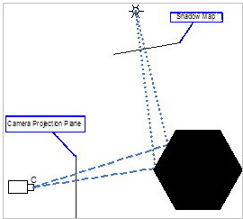
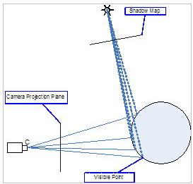
Figure 2: Difference in angle between rendered scene and shadow map. In the above diagram, the portion of the rendered scene has a larger footprint on the camera's projection plane than the light's projection plane. The size disparity means that multiple pixels in the rendered output will be mapped back to a single pixel in the shadow map. The discreet samples of the shadow map can also cause incorrect self-shadowing when the final point rendered is not close enough to the sample in the shadow map. A bias value can be added to the test to alleviate some of the problem, but if the bias value is increased too much, the shadow test will fail incorrectly and create visible gaps when an occluder and a receiver meet.
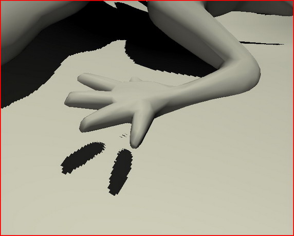
Figure 3: An illustration of poor self shadowing, jagged shadow boundaries, and gap in projected shadow. The shadow map used for the picture above does not match well with the camera's position. The low resolution causes the jagged shadow boundaries. The z-bias needed to compensate for lack of precision in the z-buffer precision causes the gaps in the shadow caused by the foot where it is too close to the receiver.
Solutions
Several new algorithms for generating shadow maps have been developed with the goal of removing some or all of the aliasing that has plagued the shadow map technique. The techniques all attempt to change the resulting depth map sample positions to more closely match the samples required for the final rendering.
Perspective Shadow Maps
Perspective shadow maps change the sampling for the shadow map by first transforming from world to camera perspective space [Stamminger and Drettakis 2002]. The perspective transformation maps the world space view frustum into a unit cube which makes objects close to the camera larger. Then, when the shadow map is created from the light's perspective, more of the space in the shadow map is devoted to the geometry that is closer to the camera.
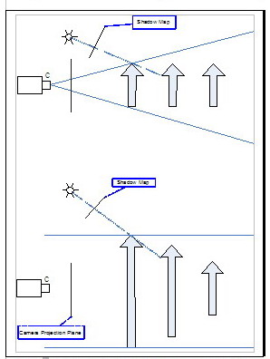
Figure 4: Scene before and after the camera's perspective transformation. After the perspective transformation, object closer to the camera will appear larger and will use more of the shadow map area. Unfortunately, the camera's perspective transformation adds a few complications. The light space is changed by the transform and requires some care when creating the actual shadow map. A directional light becomes point light, but the light will point in the opposite direction if it is behind the camera. Point lights behave similarly and a point light behind the camera is inverted. Point lights in the same plane as the camera become directional lights. In addition to the light changes, occluders that are outside the view frustum must also be included. Occluders behind the camera are mapped beyond the infinity plane causing the occluder to appear behind all geometry. Stamminger and Drettakis provide a work-arounds for dealing with post-perspective space in the original paper, and Simon Kozlov provides a number of additional refinements of the perspective shadow map technique [Kozlov 2004].
Scene Optimized Shadow Maps
Scene optimal shadow maps present the problem of shadow map aliasing as a classical optimization problem [Chong and Gortler 2006]. The goal is to minimize the ratio of screen space area to shadow space area, or conversely, maximize the number of shadow map texels per screen pixel. Instead of transforming the world before creating the shadow map as perspective shadow maps do, scene optimal shadow maps modify the transform used when creating the shadow map. Although implementation is more involved, the end result is a good shadow map without the special cases involved in the perspective shadow maps.
Scene optimal shadow maps modify the optical axis and the angle of the projection plane to warp the scene when creating the shadow map to better match the sampling requirements for the final scene. Scene optimal shadow maps require three steps. First, the scene is rendered from the camera's point of view. This stage determines the positions of all of the visible points. Next, that data is read back and used to calculate the lights projection transformation. Then the scene is rendered from the light's point of view with the projection transform determined in the previous step. Finally, the scene is rendered using the shadow map to determine shadows.
Chong and Gorlter use classical constrained optimization (gradient descent algorithm) to determine the light's perspective projection transform. First they determine the view space positions that are near shadow boundaries. They define the term to minimize as rate of change in screen space coordinates relative to the rate of change in light space coordinates. They report that only three iterations were required to reach a suitably optimized transform.
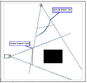
Figure 5: Scene Optimal Shadow Map. For scene optimal shadow maps, the projection plane is warped and angled so that the shadow map has more samples associated with the visible pixels in the final scene. Scene optimized shadow maps have two possible weaknesses. First, the read back of the rendered scene could be too expensive for some applications. Second, as the camera moves through the scene, the optimal shadow map will change and can cause some artifacts near the shadow boundaries.
Logarithmic Shadow Maps
Logarithmic shadow maps are another more extreme approach to modifying the light's viewing transformation [Lloyd 2007]. The goal is to distribute the shadow map sampling space more evenly over the scene. The logarithmic shadow map representation makes the projected z value vary more consistently (figure 6). The changes in the perspective means that the sample points on an object, a ground plane for example, as it extends away from the viewer, are spaced more evenly along the object as opposed to being bunched together near the viewer. Then when the shadow map is accessed as the final scene is rendered, the shadow map sample points will be more evenly distributed over a larger part of the scene.
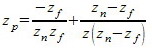
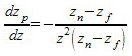
Projection type Transformed z value Rate of change Perspective
 Logarithmic

Figure 6: Comparison of perspective and logarithmic projection. The logarithmic projection has a higher rate of change and so the logarithmic shadow maps have more uniform sampling. Logarithmic shadow maps require changes to the rasterization stage of the pipeline because it is not a linear transformation. On a logarithmic shadow map, straight lines may become curved lines; so, testing if a sample point is inside a triangle becomes more complicated. Additionally, while standard transformation and rasterization require multiplications, logarithmic shadow maps require more expensive exponential calculations.
Irregular Z-Buffer and Alias-Free Shadow Maps
Irregular Z-Buffer [Johnson et al. 2004] and Alias-Free Shadow Maps [Aila and Laine 2004] propose similar modifications to the standard shadow map algorithm that requires changes to the rasterization stage when creating the shadow map. During the standard rasterization stage, sample points are arrayed in a uniform grid with one sample point corresponding to the center of each pixel. The methods above attempt to modify the projection and perspective transformations to make better use of the uniform sample points. The irregular z-buffer algorithms create a 1:1 correspondence between the visible geometry in the final rendered scene and the sample points in the shadow map by using a non-uniform collection of sample points.
The first stage of the irregular z-buffer algorithm is to render the scene from the camera's point of view. The rendered output is read back, and all visible points are then transformed from their world positions to the lights view plane. The scene is then rendered from the point of view of the light with the points on the view plane serving as the sample points for rasterization. Now the shadow map has perfect sample for the points visible from the camera so there is no shadow aliasing.
Irregular Z-buffer Sampling. For the Irregular Z-buffer, the scene is rendered for the camera's point of view to determine the visible points. These points are then projected back to the light to determine the sample points for the final shadow map. There is a 1:1 mapping between the visible points in the final scene and the sampled points in the shadow map. Of course, current hardware is designed for the uniformly distributed sample points for rasterization. Johnson et al. focus on an algorithm and data structures that target a possible hardware implementation. Aila and Laine use a software rasterizer and take advantage flexibility that that allows.
Recently, graphics vendors have increased the flexibility and programmability of their hardware. As graphics standards allow greater flexibility to developers and/or the tools to program the hardware become more advanced and, the irregular z-buffer will be available for real-time applications, and, once available, additional refinements and applications can be explored.
Conclusion
Algorithm Hardware support View dependent Perspective Shadow Maps Yes No Scene Optimized Shadow Maps Yes Yes Logarithmic Shadow Maps No No Irregular Z-buffer No Yes
Figure 8: Brief comparison of the shadow map algorithms. Shadow maps are a good, straight-forward algorithm for generating shadows. Very recent and significant changes, such as scene optimized shadow maps, alleviate the aliasing problems that have limited the utility of shadow maps while maintaining most of the simplicity of the original algorithm. Future developments with rasterization may allow efficient implementations of the irregular shadow maps and the elimination of aliasing altogether.
References
Timo Aila and Samuli Laine, "Alias-Free Shadow Maps," Eurographics Symposium on Rendering 2004.
Hamilton Y. Chong and Steven Gortler, "Scene Optimized Shadow Mapping," Harvard Computer Science Technical Report: TR-11-06, May 2006.
Gregory S. Johnson, William R. Mark, and Christopher A. Burns, "The Irregular Z-Buffer and its Application to Shadow Mapping," The University of Texas at Austin, Department of Computer Sciences Technical Report TR-04-09, April 15, 2004.
Simon Kozlov "Perspective Shadow Maps: Care and Feeding," GPU Gems. Ed. Randima Fernando. Addison-Wesley Professional. 2004. 217-244.
Brandon Lloyd, Naga Govindaraju, David Tuft, Steve Molnar, and Dinesh Manocha, Logarithmic Shadow Maps. Retrieved March 26, 2007, from University of North Carolina GAMMA Research Group Web Site: http://gamma.cs.unc.edu/logsm, 2006.
Marc Stamminger and George Drettakis, "Perspective Shadow Maps," ACM Transaction on Graphics (SIGGRAPH 2002), vol. 21, no. 3, 2002, pp. 557--562.
Lance Williams, "Casting Curved Shadows on Curved Surfaces," Computer Graphics (SIGGRAPH 1978), vol. 12, no. 3, 1978, pp. 39--42.
