Note
The theoretical parts of this article require some knowledge of optics and electromagnetism, however the conclusion and final result (a practical implementation of single-layer thin film interference in the context of a BRDF) do not. You may therefore wish to skip the theoretical sections.
Introduction
Wave interference of light has been neglected for a long time in computer graphics, for multiple reasons. Firstly, it is often insignificant and can be cheaply approximated, or even ignored completely. Secondly, it is harder to understand as it requires interpreting light as waves instead of particles (photons). However, interference crops up almost everywhere in daily life, and has recently gained popularity in rendering applications. Examples of wave interference of light are soap bubbles, gasoline rainbow patterns, lens flares, basically everything that looks cool and/or involves multicolor patterns. For instance, in computer graphics, soap bubbles were in the past approximated with more or less realistic multicolor textures slightly panned with view angle. But it turns out that they are not that computationally difficult to accurately render. We will learn how. This article will focus on one particular form of interference, namely thin film interference. This occurs when one or more very thin transparent coatings ("films") are placed on top of a material. The films are so thin that when a light wave comes into contact with these film layers, it reflects and refracts multiple times inside the layer system, and interferes with itself in the process.
The goal is to calculate the amount of light reflected off the layer system, and the amount of light transmitted into the internal medium. We will make the assumption that no light is absorbed, which is not required but makes the calculations more approachable as considering absorption of light involves delving deep into Maxwell's equations (the behaviour of electromagnetic waves at interfaces of lossy media is nontrivial). Though in general, each layer is so thin that absorption effects can be neglected most of the time. We will derive a physical solution for the case where only one film is present (single-layer) and conclude on how to solve the general case with arbitrarily many layers. The single-layer case is sufficient to render most real life occurrences of thin-film interference, however using more layers enables many more advanced effects. The cost of calculating reflection and transmission coefficients is linear in the number of layers.
Derivation
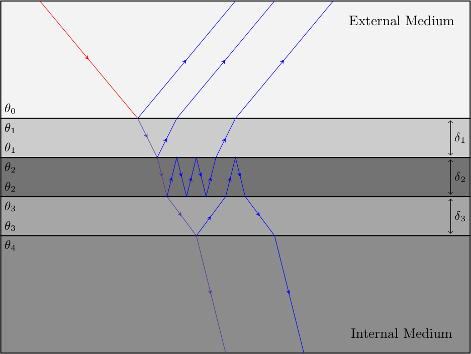
Consider a light wave incident to a thin layer of depth \(\delta\) and real refractive index \(n_1\). The external medium has refractive index \(n_0\) and the internal medium has refractive index \(n_2\). The incident angle made by the incident light wave and the film's surface normal is \(\theta_0\), the angle inside the layer is \(\theta_1\) and the refracted angle (inside the internal medium) is denoted \(\theta_2\). We will also give numbers to each of the three media: medium 0 is the external medium, medium 1 is the layer, and medium 2 is the internal medium. Also, naturally, medium 0 has to have a different refractive index than medium 1, and the same goes for medium 1 and medium 2. Media 0 and 2 can be the same, of course.
First, we know from Snell's Law that the following holds:
\[n_0 \sin{\theta_0} = n_1 \sin{\theta_1} = n_2 \sin{\theta_2}\]
Therefore the angles \(\theta_1\) and \(\theta_2\) can be derived from \(\theta_0\). Now, we see from the diagram that the only path the light wave can follow is a zigzag pattern as it bounces back and forth between the layer, until it gets transmitted either back into the external medium or into the internal medium.
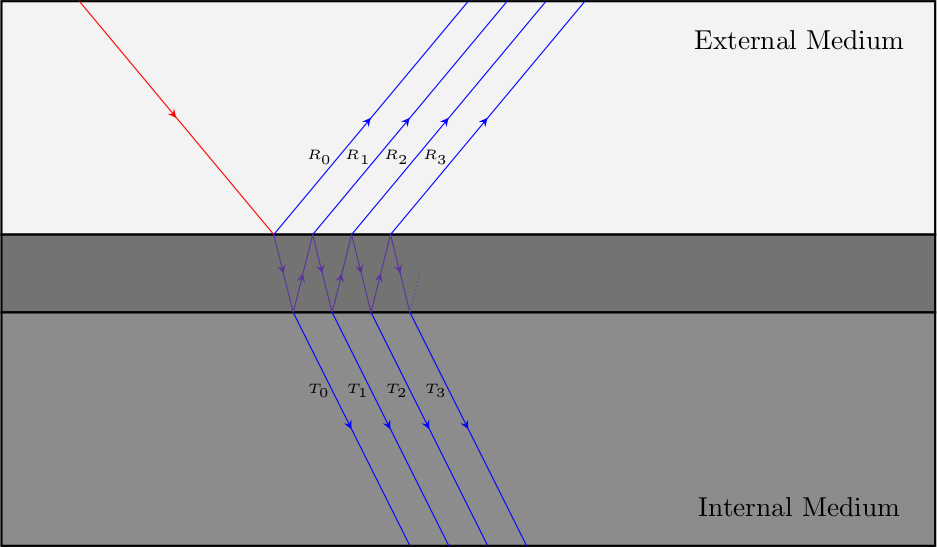
We also note that all the reflected waves (denoted \(R_0\), \(R_1\), ...) and all the transmitted waves are parallel. This is necessary for interference and is a natural consequence of the reciprocal nature of Snell's Law. And we have assumed that the media involved are non-absorbing, therefore by conservation of energy the reflection and transmission coefficients must sum up to exactly one. It turns out that it is slightly easier to derive the transmission coefficient, so we will do that, but we would get the same thing either way.
The reason for this is because the very first reflected wave \(R_0\) does not actually penetrate the layer, which means it needs to be handled separately. This does not occur for transmitted waves.
Now let's take a look at what happens to the amplitude of the light wave as it travels through this layer system. First, we need to introduce the Fresnel equations, which let us calculate how much of a light wave's amplitude is reflected and how much of it is transmitted whenever it comes into contact with an interface. These equations should be familiar, although perhaps not in the following form:
\[r_s = \frac{n_i \cos{\theta_i} - n_j \cos{\theta_j}}{n_i \cos{\theta_i} + n_j \cos{\theta_j}}\] \[t_s = \frac{2 n_i \cos{\theta_i}}{n_i \cos{\theta_i} + n_j \cos{\theta_j}}\] \[r_p = \frac{n_j \cos{\theta_i} - n_i \cos{\theta_j}}{n_i \cos{\theta_j} + n_j \cos{\theta_i}}\] \[t_p = \frac{2 n_i \cos{\theta_i}}{n_i \cos{\theta_j} + n_j \cos{\theta_i}}\]
These are amplitude reflection/transmission coefficients, for s-polarized and p-polarized light. Indeed, light polarization is important, and in the derivation we will assume the light wave has a given known polarization. We will now introduce some notation. The following denotes the amplitude reflection coefficient for a light wave going from medium \(i\) to medium \(j\):
\[\rho_{i | j} = r_{s/p}\]
Where the correct reflection coefficient is chosen based on the light wave's polarization. Similarly, the amplitude transmission coefficient is:
\[\tau_{i | j} = t_{s/p}\]
Because the refractive indices and incident angles for each medium are known and constant, we do not need to specify them. We are now ready to tackle the problem. Consider the transmitted wave \(T_0\). It's easy to see that since it crosses the layer at two locations, and never reflects anywhere, its amplitude will be:
\[\tau_{0 | 1} \tau_{1 | 2}\]
What about the second transmitted wave \(T_1\)? This one is transmitted once from medium 0 to medium 1, reflects off the medium 1 to medium 2 interface, is reflected again from the medium 1 to medium 0 interface, and is finally transmitted across the medium 1 to medium 2 interface. So its amplitude will be:
\[\tau_{0 | 1} \rho_{1 | 2} \rho_{1 | 0} \tau_{1 | 2} = \tau_{0 | 1} \tau_{1 | 2} \rho_{1 | 0} \rho_{1 | 2}\]
We can see there's a pattern here. Every successive transmitted wave will simply reflect two additional times off the top and bottom interface. So, if we denote the amplitude of the \(k\)th transmitted wave \(A_k\), we have:
\[A_k = \tau_{0 | 1} \tau_{1 | 2} \rho_{1 | 0}^k \rho_{1 | 2}^k\]
We note that even though there are (in theory) infinitely many transmitted waves, their amplitude decreases exponentially, since the Fresnel amplitude reflection coefficient is never quite 1 (except in the case of total internal reflection, where all light is reflected and none is transmitted, of course, if this is the case then the incident wave fully reflects off the layer first chance it gets and so this analysis doesn't apply).
We now have the amplitudes of each transmitted wave. Can we calculate the total amount of transmitted light now? Not quite. These are waves, and you can't just add waves using their amplitudes. We need to consider the phase of each transmitted wave, as these waves might cancel each other out depending on their phase (out of phase waves cancel out, in phase waves amplify each other).
The waves also have a frequency, but the frequency depends only on the incident wave's wavelength, which is known and constant, so it can be taken out of the equation. How do we calculate the phase of each transmitted wave? This is in fact a simple textbook thin film interference problem, and if we denote the phase of the \(k\)th transmitted wave \(\varphi_k\), the following holds:
\[\varphi_k = k \left [ \frac{2 \pi}{\lambda} \left ( 2 n_1 \delta \cos{\theta_1} \right ) + \Delta \right ]\]
Where \(\lambda\) is the light wave's wavelength and \(\Delta\) is a constant meant to account for phase changes upon reflection (we will expand on this soon). The important thing is that the phase of every transmitted wave is a multiple of a constant (with respect to the wave index \(k\))! That is:
\[\varphi_k = k \left [ \frac{2 \pi}{\lambda} \left ( 2 n_1 \delta \cos{\theta_1} \right ) + \Delta \right ] = k \varphi\]
The explanation for this lies in the rather trivial observation that the distance travelled by the light wave inside the layer increases by a constant factor for every consecutive transmitted wave. This is fortunate, as it makes the upcoming calculations very simple. Had the phase depended on \(k\) in a more complicated way, the problem could have very well been analytically intractable.
We will now explain the meaning of the \(\Delta\) term. When a wave (any wave, not just electromagnetic light waves) reflects off a medium denser than the one it is in, it will undergo a 180-degree phase change. Because the refractive index is a measure of how dense a medium is, we can use that to calculate this constant. There are two possible reflections here: one at the top interface and one at the bottom interface. We denote:
\[\Delta_{i | j} = \begin{cases} 0 ~ & \text{if} ~ n_i > n_j \\ \pi ~ & \text{if} ~ n_i < n_j \end{cases}\]
For the reflection phase change when reflecting off the interface from medium \(i\) to medium \(j\). Therefore, we see that:
\[\Delta = \Delta_{1 | 0} + \Delta_{1 | 2}\]
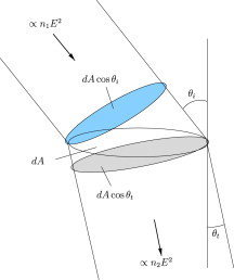
Which is constant, as it depends only on the refractive indices of each medium. At this point we have the amplitude and phase of each transmitted wave. All we have to do is sum them up (as waves), and take the squared magnitude of the resulting complex amplitude to obtain the transmitted intensity. However, because the transmitted waves are in a different medium than the incident wave, we need to take into account the ratio of beam surface area to make sure energy is conserved. That is, we need to multiply by:
\[\frac{n_2 \cos{\theta_2}}{n_0 \cos{\theta_0}}\]
This is actually two factors in one. The first, ratio of refractive indices, is there because the transmitted wave won't, in general, have the same speed as the incident wave (for instance, light travels slower in water than in air). So the perceived intensity will not be the same. Remember, intensity is energy per second per squared area, so if the wave is faster the intensity will be higher, so we need to scale the intensity down by a corresponding amount to make sure energy is conserved. The second factor, ratio of cosines, exists because of the change in area of a beam of light as it is refracted. The following diagram illustrates all of this nicely:
It is worth noting that reflected light is treated the same, however because reflected waves remain in the same medium and the reflected angle is the same as the incident angle, both ratios just cancel out. Now, we have the following expression for the transmitted intensity:
\[I_T = \frac{n_2 \cos{\theta_2}}{n_0 \cos{\theta_0}} \left | \sum_{k = 0}^\infty A_k e^{i \varphi_k} \right |^2\]
This looks complicated, but it actually isn't. This is because both the phase and the amplitude are dependent on \(k\) in such a way that:
\[I_T = \frac{n_2 \cos{\theta_2}}{n_0 \cos{\theta_0}} \left | \sum_{k = 0}^\infty \tau_{0 | 1} \tau_{1 | 2} \rho_{1 | 0}^k \rho_{1 | 2}^k e^{i k \varphi} \right |^2 = \frac{n_2 \cos{\theta_2}}{n_0 \cos{\theta_0}} \left | \tau_{0 | 1} \tau_{1 | 2} \sum_{k = 0}^\infty \left ( \rho_{1 | 0} \rho_{1 | 2} e^{i \varphi} \right )^k \right |^2\]
And we will now use the following two substitutions, just to make the expressions a bit more readable:
\[\alpha = \rho_{1 | 0} \rho_{1 | 2}\] \[\beta = \tau_{0 | 1} \tau_{1 | 2}\]
We now have a geometric series sum, which we can evaluate as follows:
\[I_T = \frac{n_2 \cos{\theta_2}}{n_0 \cos{\theta_0}} \left | \beta \sum_{k = 0}^\infty \left ( \alpha e^{i \varphi} \right )^k \right |^2 = \frac{n_2 \cos{\theta_2}}{n_0 \cos{\theta_0}} \left | \frac{\beta}{1 - \alpha e^{i \varphi}} \right |^2\]
Simplifying rather elegantly to the following (assuming \(\alpha\) is real):
\[I_T = \left ( \frac{n_2 \cos{\theta_2}}{n_0 \cos{\theta_0}} \right ) \frac{|\beta|^2}{| \alpha |^2 - 2 \alpha \cos{\varphi} + 1}\]
And by conservation of energy, we have:
\[I_T + I_R = 1\]
Which concludes the derivation. As a final note, we can calculate the average over all possible phases of this result. If we are correct, then we should get the same result as a geometric optics derivation. The reader can verify that, indeed, we have:
\[\overline{I_T} = \frac{1}{2 \pi} \int_{-\pi}^{+\pi} I_T ~ \text{d} \varphi = \left ( \frac{n_2 \cos{\theta_2}}{n_0 \cos{\theta_0}} \right ) \frac{|\beta|^2}{1 - |\alpha|^2}\]
We conclude that the transmission coefficient (intensity of light transmitted across the layer) is \(I_T\) and the reflection coefficient (intensity of light reflected off the layer) is \(I_R\).
General Case
The derivation shown above is quite naive, and does not generalize well at all to multiple layers, though it is the simplest method to see what is happening at a low level. If you wish to implement n-layer thin film interference, the method of choice is the Transfer-matrix method, which simplifies the problem down to a series of matrix multiplications and can be derived using powerful electromagnetism techniques.
Implementation
So we now know just how much light is reflected from the layer. How can we implement this in the context of a BRDF? It's quite simple: this reflected term simply replaces the ordinary Fresnel term, accounting for thin film interference effects. This means you can trivially include thin-film interference effects in any BRDF as long as it has a Fresnel term. The function below computes the reflection coefficient for a given wavelength and incident angle.
// cosI is the cosine of the incident angle, that is, cos0 = dot(view angle, normal)
// lambda is the wavelength of the incident light (e.g. lambda = 510 for green)
float ThinFilmReflectance(float cos0, float lambda)
{
    const float thickness; // the thin film thickness
    const float n0, n1, n2; // the refractive indices

    // compute the phase change term (constant)
    const float d10 = (n1 > n0) ? 0 : PI;
    const float d12 = (n1 > n2) ? 0 : PI;
    const float delta = d10 + d12;

    // now, compute cos1, the cosine of the reflected angle
    float sin1 = pow(n0 / n1, 2) * (1 - pow(cos0, 2));
    if (sin1 > 1) return 1.0f;

    // total internal reflection
    float cos1 = sqrt(1 - sin1);

    // compute cos2, the cosine of the final transmitted angle, i.e. cos(theta_2)
    // we need this angle for the Fresnel terms at the bottom interface
    float sin2 = pow(n0 / n2, 2) * (1 - pow(cos0, 2));
    if (sin2 > 1) return 1.0f;

    // total internal reflection
    float cos2 = sqrt(1 - sin2);

    // get the reflection transmission amplitude Fresnel coefficients
    float alpha_s = rs(n1, n0, cos1, cos0) * rs(n1, n2, cos1, cos2);

    // rho_10 * rho_12 (s-polarized)
    float alpha_p = rp(n1, n0, cos1, cos0) * rp(n1, n2, cos1, cos2);

    // rho_10 * rho_12 (p-polarized)
    float beta_s = ts(n0, n1, cos0, cos1) * ts(n1, n2, cos1, cos2);

    // tau_01 * tau_12 (s-polarized)
    float beta_p = tp(n0, n1, cos0, cos1) * tp(n1, n2, cos1, cos2);

    // tau_01 * tau_12 (p-polarized)
    // compute the phase term (phi)
    float phi = (2 * PI / lambda) * (2 * n1 * thickness * cos1) + delta;

    // finally, evaluate the transmitted intensity for the two possible polarizations
    float ts = pow(beta_s) / (pow(alpha_s, 2) - 2 * alpha_s * cos(phi) + 1);
    float tp = pow(beta_p) / (pow(alpha_p, 2) - 2 * alpha_p * cos(phi) + 1);

    // we need to take into account conservation of energy for transmission
    float beamRatio = (n2 * cos2) / (n0 * cos0);

    // calculate the average transmitted intensity (if you know the polarization distribution of your
    // light source, you should specify it here. if you don't, a 50%/50% average is generally used)
    float t = beamRatio * (ts + tp) / 2;

    // and finally, derive the reflected intensity
    return 1 - t;
}
We can now sample this function at red, green, and blue wavelengths (650, 510, 475 nanometers, respectively) and substitute the RGB reflectance obtained into the Fresnel term of the BRDF. Or, if you are rendering spectrally, just give the wavelength directly. That's it. One word on polarization - in general, in computer graphics, we assume light contains an equal amount of s-polarized and p-polarized light waves. Then the Fresnel reflection coefficient is simply an average between the s-polarized and p-polarized light reflection coefficients, as the comment indicates. If you have more information on how much s-polarized light is emitted by your light source, then the average should reflect that.
BRDF Explorer Sample
The following shader script implements the BRDF in the Disney BRDF Explorer tool, using the stock Blinn-Phong shader with the default microfacet distribution. Note how we just implemented the code separately and multiplied the BRDF by the modified "thin film" Fresnel term.
 analytic
# Blinn Phong based on halfway-vector with single-layer thin
# film wave interference effects via a Fresnel film coating.
::begin parameters
    float thickness 0 3000 250 # Thin film thickness (in nm)
    float externalIOR 0.2 3 1 # External (air) refractive index
    float thinfilmIOR 0.2 3 1.5 # Layer (thin film) refractive index
    float internalIOR 0.2 3 1.25 # Internal (object) refractive index
    float n 1 1000 100 # Blinn-Phong microfacet exponent
::end parameters

::begin shader
    const float PI = 3.14159265f;

    /* Amplitude reflection coefficient (s-polarized) */
    float rs(float n1, float n2, float cosI, float cosT)
    {
        return (n1 * cosI - n2 * cosT) / (n1 * cosI + n2 * cosT);
    }

    /* Amplitude reflection coefficient (p-polarized) */
    float rp(float n1, float n2, float cosI, float cosT)
    {
        return (n2 * cosI - n1 * cosT) / (n1 * cosT + n2 * cosI);
    }

    /* Amplitude transmission coefficient (s-polarized) */
    float ts(float n1, float n2, float cosI, float cosT)
    {
        return 2 * n1 * cosI / (n1 * cosI + n2 * cosT);
    }

    /* Amplitude transmission coefficient (p-polarized) */
    float tp(float n1, float n2, float cosI, float cosT)
    {
        return 2 * n1 * cosI / (n1 * cosT + n2 * cosI);
    }

    /* Pass the incident cosine. */
    vec3 FresnelCoating(float cos0)
    {
        /* Precompute the reflection phase changes (depends on IOR) */
        float delta10 = (thinfilmIOR < externalIOR) ? PI : 0.0f;
        float delta12 = (thinfilmIOR < internalIOR) ? PI : 0.0f;
        float delta = delta10 + delta12;

        /* Calculate the thin film layer (and transmitted) angle cosines. */
        float sin1 = pow(externalIOR / thinfilmIOR, 2) * (1 - pow(cos0, 2));
        float sin2 = pow(externalIOR / internalIOR, 2) * (1 - pow(cos0, 2));

        if ((sin1 > 1) || (sin2 > 1)) return vec3(1);

        /* Account for TIR. */
        float cos1 = sqrt(1 - sin1), cos2 = sqrt(1 - sin2);

        /* Calculate the interference phase change. */
        vec3 phi = vec3(2 * thinfilmIOR * thickness * cos1);
        phi *= 2 * PI / vec3(650, 510, 475); phi += delta;

        /* Obtain the various Fresnel amplitude coefficients. */
        float alpha_s = rs(thinfilmIOR, externalIOR, cos1, cos0) * rs(thinfilmIOR, internalIOR, cos1, cos2);
        float alpha_p = rp(thinfilmIOR, externalIOR, cos1, cos0) * rp(thinfilmIOR, internalIOR, cos1, cos2);
        float beta_s = ts(externalIOR, thinfilmIOR, cos0, cos1) * ts(thinfilmIOR, internalIOR, cos1, cos2);
        float beta_p = tp(externalIOR, thinfilmIOR, cos0, cos1) * tp(thinfilmIOR, internalIOR, cos1, cos2);

        /* Calculate the s- and p-polarized intensity transmission coefficient. */
        vec3 ts = pow(beta_s, 2) / (pow(alpha_s, 2) - 2 * alpha_s * cos(phi) + 1);
        vec3 tp = pow(beta_p, 2) / (pow(alpha_p, 2) - 2 * alpha_p * cos(phi) + 1);

        /* Calculate the transmitted power ratio for medium change. */
        float beamRatio = (internalIOR * cos2) / (externalIOR * cos0);

        /* Calculate the average reflectance. */
        return 1 - beamRatio * (ts + tp) * 0.5f;
    }

    vec3 BRDF(vec3 L, vec3 V, vec3 N, vec3 X, vec3 Y)
    {
        vec3 H = normalize(L + V);
        float val = pow(max(0, dot(N, H)), n);
        return vec3(val) * FresnelCoating(dot(V, H));
    }

    ::end shader
It is worth noting that this is a reference implementation meant to be readable, and can be thoroughly optimized. In particular, the Fresnel calculations are the most expensive, but there are numerous ways of reducing the amount of computations. For instance, we can use the reciprocity properties of s-polarized light, and also recycle many intermediate calculations.
If you are not interested in perfect physical accuracy, you can also skip the polarization calculations and directly use intensity Fresnel coefficients, though because amplitudes are signed and intensities are not, you will need to calculate the proper sign to use for the cosine term somehow (or just ignore it altogether and have incorrect but plausible thin film interference).
If you are really desperate about runtime performance, you can still retain the nice colorful patterns while trading physical accuracy by approximating the final formula however you see fit, the only fundamental requirement is that the \(\cos{\varphi}\) term be in there somewhere. This is a screenshot of the above BRDF's polar plot at incidence 45 degrees and illustrates its wavelength-dependent nature:
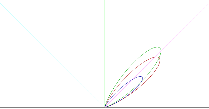
Note how the BRDF differs for the three channels (in fact, every wavelength produces a different response, but we're working in RGB mode here). And here are a few renders (still from BRDF Explorer) with some sensible parameters. Here we assume the internal medium is fully opaque:
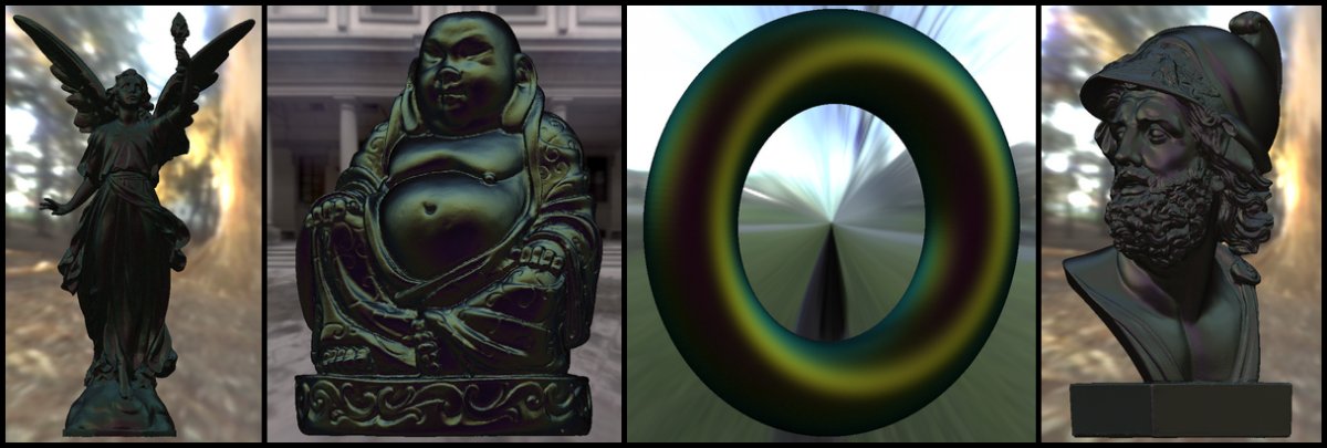
What happens when we set the thin film thickness to zero? In this case, the layer physically disappears and the formula degenerates to ordinary Fresnel reflection (more specifically, the Fresnel reflection coefficients for the layer become zero while the transmission coefficients become one). What about making the thin film extremely thick?
In that case, we see that the rate of change of the phase \(\varphi\) with respect to view angle becomes arbitrarily large, causing the interference effects to average out to white light, as expected. Also, because we are using a BRDF, we are assuming that light exits the surface at the same point it enters it, which is a very good approximation when the thin film is very small (on the order of light's wavelength). However, as the film becomes thicker, the approximation breaks down, so the film should probably be no larger than a few thousand nanometers, at most.
The same holds true for microfacet distributions. Thin films coated over surfaces with very high microfacet roughness coefficients are somewhat unphysical, since a coating naturally tends to be smoother than the surface it is applied on. This should be kept in mind, as the two layer interfaces are assumed to be coplanar.
You might also wonder what happens if refractive index depends on wavelength. Well, not much, the correct refractive index and incident/transmitted angles are simply used, and everything else remains the same, since waves of different frequencies do not interfere in any meaningful way. The BRDF above chooses to assume a constant IOR, though, to simplify matters. Also, if the refractive indices are wavelength-dependent, you will also observe dispersion effects in the transmitted light.
Transparency?
You may also want to handle transparency if the internal medium is not opaque. You can use whatever method you already have in place to render refractive surfaces, using the final transmitted angle (cos2 in the pseudocode). This is necessary for soap bubbles. Of course, if the internal medium is opaque, this is not necessary as the transmitted light is simply absorbed.
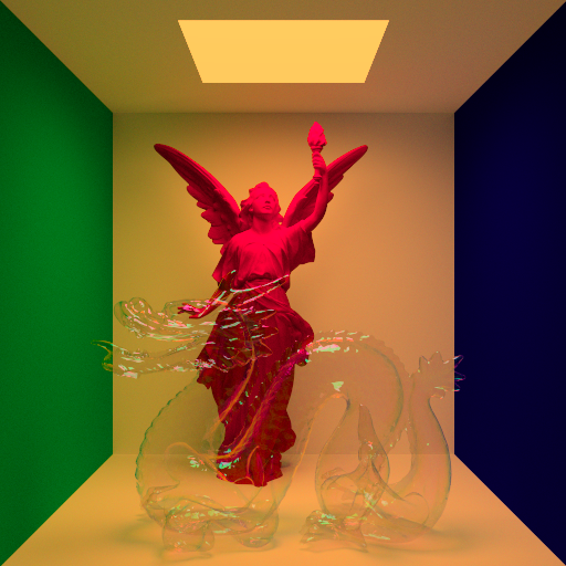
It is also possible to use this with subsurface scattering (thus representing a subsurface scattering material with a thin film coating) by using the transmitted light (suitably refracted, as mentioned above). Here is a render of a model with a soap-bubble-like BRDF, rendered with ray tracing. In this case, there is no visible refraction because soap bubbles are simply an air/water/air interface, so the final transmitted angle is the same as the incident angle:
Final notes
A good selection of parameters is essential to obtain realistic results. For instance, the film thickness should be on the order of light's wavelength (a few hundred nanometers). As you increase the thickness, interference effects disappear and as the thickness tends to zero, you just get ordinary Fresnel reflection, as mentioned previously.
Make sure to use correct refractive indices for your materials. The range of values which can produce interference effects is quite narrow, so the parameters have to be accurate.
For metals or materials where the refractive index varies considerably over the visible spectrum, such as copper, three refractive indices (one per RGB channel) should be used for physical accuracy if possible. This requires only minor changes to the BRDF, as everything can be vectorized. It suffices to make the IOR parameters 3-component vectors and vectorize the Fresnel coefficient functions. The computational cost is therefore exactly the same.
One last point is that for non-solid thin films, such as oil or water coatings, the thickness of the layer is probably not constant at every point of a given object. As an example, soap bubbles are thicker at the bottom than at the top, due to gravity. For a convincing render, this should be taken into account.
As a result, thin film thickness should probably be a vertex attribute rather than a material attribute, or, alternatively, a more general reflectance model should be considered (such as a spatially varying BRDF). Adding some noise to the film thickness can also go very far in improving the appearance of some materials, and it is convenient to implement. Attached is the zipped BRDF Explorer script so that you may play around with it at your leisure.
Article Update Log
26 Aug 2013: Converted all externally linked formulas to actual LaTeX code, removed now redundant images.
2 May 2013: Fixed a couple of bugs in the shader, corrected a few typos and improved formatting.
30 Apr 2013: Added some notes about interesting variations to apply to film thickness and on optimizations.
29 Apr 2013: Added notes on the motivation of neglecting absorption effects.
28 Apr 2013: Added notes on IOR and physical accuracy of solution.
27 Apr 2013: Added extra render, improved formatting.
26 Apr 2013: Added BRDF and some renders.
25 Apr 2013: Began writing article.


")
Great article! Obviously there's lots of math to cover in such a short article. I would love to dig deeper into these equations. I thought you presented the high level details very well. As only a second year University student, you have an impressive understanding of this material. Did you teach yourself most of this stuff?
I started young myself (I'm just graduating University), but I only recently began digging into the more theoretical and challenging math behind graphics. At any rate, nice job!