Introduction
Spheres are among the most common geometric entities used in performing various game engine related tasks such as object culling, containment, bounding volumes and bounding volume hierarchies to name a few.

Spheres are excellent candidates for bounding volumes and are widely used mainly because they have inexpensive intersection tests, are easy to transform (they are rotation-invariant) and have small memory usage.

Unfortunately, axis-aligned bounding boxes are often preferred over spheres due to fitting problems or the fact that a tight fitting sphere is hard to compute in real time. In this article we'll explore what is considered the optimal solution to the sphere fitting problem, a solution proposed by Emo Welzl [Welzl91]. For simplicity we'll limit ourselves to the discussion and implementation of the algorithm in 2D only, although the algorithm scales quite nicely to 3D.

A simple Java-based implementation of the sphere generation algorithm is provided. The code is described later on in the article.


The problem of finding an optimal sphere
There are many algorithms to compute an enclosing sphere of a set of points. Most of the algorithms may be easy to implement and understand but fail to provide optimal spheres in most cases.

A description of some of the basic algorithms and their shortcomings is listed below:

• The mean of the input points - This very simple and linear algorithm is the simplest of all but can give extremely bad results due to point clustering. The sphere can have up to twice the optimal radius. Clearly this is not the way to go.
• A sphere contained within an AABB - A simple approximation is to find the AABB enclosing all points and obtaining the midpoint (the sphere's center) and the radius to be the distance from this center to the farthest point. While this approach is fairly simple and provides adequate results, it does not compare to the optimal solution.
• Computing a sphere using maximum spread - This approach attempts to find the axis direction of the maximum spread of the input points and uses it as the diameter of the sphere. The points most extreme on the axis are selected and the center is set halfway between them. Although an interesting approach, it suffers from problems due to point clustering and internal points ruining the covariance.
• Brute force - Since a sphere in 3D is uniquely defined by four points (two in 2D), a simple brute force approach might attempt to find the minimum sphere by trying all combination of spheres made up by four points, three points and two points, keeping the minimum-sized sphere that contains all points. This approach is the worst with a running complexity of O(n5).

The optimal solution
A better solution to the problem is to grow a sphere to contain all the input points. The solution sounds simple enough and is fairly easy to visualize. Every time the sphere is grown to contain a new point, the sphere is updated. Points that were inside the sphere might find themselves outside the new sphere since the center and the radius might both change.

For this reason, the algorithm is restarted and the input points are tested against the sphere again. Any point that lies within it is ignored, while a point that lies outside will trigger a new update just as before. A new point P will then cause the sphere to grow and include P.

Visually the two cases before and after the update might look like this:

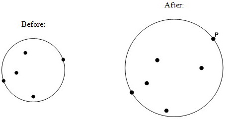The circle on the left represents the sphere before it was updated with point P. The sphere is currently defined by only two points but it is clearly the optimal sphere containing all the points at this time (a sphere in 2D is uniquely defined by three points, four in 3D so there is no need for more than three).

Once a new point P is introduced, the sphere should grow to contain the new point. Since there is no logic in growing the sphere more than necessary, point P is considered to be on the sphere itself. On the right we can see the new sphere, now defined by P and the left-most point from the earlier case.

Growing the sphere is not a trivial operation. In fact, by just making the radius larger and not changing the center, the new sphere will not be optimal as the left-most point (that was on the sphere itself) will no longer be on it but inside it.

In order to prevent this and find an optimal sphere the algorithm defines a support set that contains points (called support points). Supporting points are defined as points that lie on the sphere perimeter (lie on the sphere). In the smaller sphere there were two supporting points. After the sphere has grown we have to add point P to the support points (since it is on the sphere) and recalculate the sphere from the points in the set.

Since the set after the addition now contains three points the only problem left is to find the minimum sphere from the three points and if not found, from two points, etc.

Since the number of points in the set is only three, the number of permutations to test is not large and thus we find the new optimal sphere. Note however that the new optimal sphere calculated from the set of three points may be defined by only two points. This is the case shown on the right.

When a new point was added (P), the set now contains three points but the minimum sphere is found by only using two points (one of the permutations). Therefore, one of the supporting points before the update is no longer a supporting point since it's not on the sphere and gets removed from the set.

The update procedure is therefore responsible for the following tasks:

• Add the new point P to the support set
• Compute the minimum sphere from the new set
• Any points from the set not on the sphere perimeter after the new sphere is computed are removed from the set

After the update, if the new minimum sphere is larger than the existing minimum sphere, the update was successful and the algorithm restarts in order to check all points for inclusion once again. The algorithm stops only when a sphere is found that includes all points from the input set (some lie on the sphere itself). Naturally, the algorithm's last iteration processes all the points not in the set and ignored them as being inside the sphere.


Time complexity
If the number of algorithm restarts mis effectively small compared to the number of input points, the algorithm is then considered to have a linear running time. However, if the algorithm needs to restart after every update then the running time is effectively squared, O(n2).

In order to ensure that the input points have only a small chance of being arranged in a way that gives the worst-case running time, the points are shuffled in a random order. Welzl showed that if the points have a random ordering then the algorithm runs in expected linear time, a total running time of O(m * n). It is important to note that the update process itself in which the algorithm uses the points in the support set plus the new point to find the new minimum sphere is bounded since the number of points in the set is small (a maximum of 4 in 2D and 5 in 3D) and the number of possible spheres is rather small. Since m is the number of restarts it is also the number of update operations.


The update process
Up until now we've been discussing the algorithm but assumed the update process gives the smallest enclosing sphere from the points in the set plus the new point P that was added to the set.

The update process attempts to find the smallest sphere by computing all combinations of spheres possible from the set plus the new point P, now a new set. Depending on the number of points in the set, the possible permutations for a 2D circle are (assuming the points in the set are p0, p1...):

• If the set has one point and P is added we now have two points defining the circle.
• If the set has two points and P is added we now have three points. The minimum circle can now be defined by (p0, P), (p1, P) or in case the minimum circle is not one of them, it will be defined by (p0, p1, P).
• If the set has three points and P is added we now have four possible points. The circle can be defined by: (p0, p3) if p1 and p2 are within it, (p1, p3) if p0 and p2 are within it, (p2, p3) if p0 and p1 are within it, (p0, p1, p3) if p2 is within it, (p0, p2, p3) if p1 is within it, (p1, p2, p3) if p0 is within it, for a total of six permutations (three circles defined by two points and three defined by three points)
• In 3D only - The set may contain four points when P is added to it, giving a total of five points. Since up to four points can be used to define the sphere there are a total of 14 possible permutations.

Note that we do not deal with the case where the set has no points when P is added to it since in our implementation this will be the algorithm's initial condition. Once a new optimal sphere is found from the new set of points it also uniquely determines which points should be removed from the set because they are no longer on the perimeter of the sphere - thus not support points.

For example, assume the set has three points when P is added to it. There are effectively four points to use for a total of 6 possible circles. Let's also assume that the optimal sphere out of the 6 spheres is the first permutation defined by (p0, P), where P is p3 (the set contains p0, p1, p2 and the new p3).

The new set should then become (p0, p3 = P) since the sphere was found to be defined by two points and the permutation is (p0, p3). The set is resized to a size of 2 and since p0 was already there, p3 replaces the other point that is in the set. In the same manner it is easy to understand the rest of the permutations, which points should be in the updated support set and which are removed.

The only problem left to solve is how to generate a sphere/circle from a given amount of input points. Our initial condition requires us to use one point (the set will initially contain one point). The permutations given above suggest we need a way to define spheres from two points and even three points.


Generating a sphere from a set of points
In this section I'll briefly describe the possible ways to create a sphere based on a number of points. As shown earlier we need functions to create a sphere from one, two and three input points (as well as four in 3D). These can be implemented by constructors of a sphere class or update functions to an existing sphere (to save object construction destruction).

Depending on the number of points these are the steps used to create the sphere:

• For one point the sphere's center is set to be the point and the radius is 0. This is the algorithm's initial condition.
• For two points the center is selected to be halfway between the two points, while the radius is set to be half the length of the vector connecting the points.
• For three points we define the center in barycentric coordinates:
  
  C = u0 * p0 + u1 * p1 + u2 * p2, where u0 + u1 + u2 = 1
  
  The radius is: R = |C-p0| = |C-p1| = |C-p2|.
  
  Using some algebra it is possible to get a system of two equations that are quite easily solved. The full details of the derivation are easy to find as the problem is well studied in computational geometry.
  
  A very good reference for this is "Geometric Tools for Computer Graphics" by David Eberly [Ebe03].

The tester and the source code
An implementation of the algorithm for 2D circles is given in the form of a simple Java-based tester. The tester provides a way for us to see the algorithm in action and see simple statistics about the number of point tests made (total iterations) and the number of restarts (m) of the algorithm.

To run it, issue the following command in the directory containing the JAR file:

> java -jar WelzlSphere.jar (Assuming you have your PATH environment variable set to point to java.exe) To use the tester, input the number of input points wanted and click 'Generate'. This will generate that amount of points in random locations and display them.

Once points are randomized, 'Create Sphere' can be used to initiate the sphere generation. The sphere is then displayed on screen along with the points. Once a sphere is created the algorithm statistics appear in the status bar and are left there until a new sphere is created.

The tester supports a maximum number of 10000 points. The number is chosen arbitrarily in the code.

In terms of the source code - It is a very simple implementation and not production code. Aside for a circle class that supports construction of circles from various amounts of points there are no custom classes to make the code simpler (a lack of a simple vector class meant some calculations are just inlined).

Some more notes:

• All coordinates and radii are in a logical coordinate system of a rectangular area of 10000 on 10000. They are later transformed to client-area coordinates when drawing
• Point locations are randomized in a way that makes it more likely for the entire circle to be visible. See the randomizePoints function for details.
• The actual drawing area is always a square. The smaller dimension (width or height) is used as a scale factor in order to make the transformation and drawing simpler. Naturally, if the frame is resized the points and circle have to be transformed to the center of the client-area.
• The limit of 10000 points is arbitrary and is only used to see how fast the algorithm can run
• The tester has had very little optimization. The algorithm runs as expected but with a large number of points the drawing delay is noticeable. Although it's very easy to make it run orders of magnitude faster this is not really a problem.
• All the sphere's radii are squared when the algorithm is running, to save the cost of performing a square root operation. Once the algorithm ends, the final sphere's radius is square-rooted.

Conclusion
Spheres can be a great bounding volume in collision detection and are generally great geometric entities. The algorithm described here (Welzl 1991) is an efficient approach at computing the minimum enclosing sphere of a set of points, in real time.

True, spheres and other bounding volumes can be computed in a pre-processing step but the need for a good real-time algorithm still exists (and it also helps to speed up pre-processing, whether the algorithm runs when loading a scene or when an external tool creates the bounding volume).


References
1. [Welzl91] - Smallest enclosing disks (balls and ellipsoids) "New Results and New Trends in Computer Science", (H. Maurer, Ed.), Lecture Notes in Computer Science 555 (1991) 359-370.

2. [Eberly03] - Geometric Tools for Computer Graphics by Philip J. Schneider and David H. Eberly, The Morgan Kaufmann Series in Computer Graphics and Geometric Modeling Copyright (C) 2003 by Elsevier Science (USA), Philip J. Schneider, and David H. Eberly