When working with geometry, you'll need to do some intersection tests at some point. Sometimes it's directly related to graphics, but sometimes it helps determine other useful things, like optimum paths. This article is meant to give the up-and-coming game developer a few more tools in their computational toolbox. For this article, I'm assuming you know all about vectors, points, dot and cross products. We'll cover some quick properties of polynomials, some things about some basic curves, and then go over intersection tests.
Note: In an attempt to make this article more accessible to those people uncomfortable with making code from straight math, I've added some coding tips to help you figure out how to use these methods.
Polynomials
The Stone-Weierstrass theorem states that any continuous function defined on a closed interval can be uniformly approximated as closely as desired with a polynomial function. For graphics and game development, that means that most 2D objects we deal with can be expressed as polynomials. The key to these intersection test methods is using that to our advantage.
Bezout's Theorem
In order to find all our intersection points, we need to know how many intersections there can be between 2 polynomials. Bezout's theorem states that for a planar algebraic curve of degree n and a second planar algebraic curve m, they intersect in exactly mn points if we properly count complex intersections, intersections at infinity, and possible multiple intersections. If they intersect in more than that number, then they intersect at infinitely many points, which means that they are the same curve. Bezout's theorem also extends to surfaces. A surface of degree m intersects a surface of degree n in a curve of degree mn. As well, a space curve of degree m intersects a surface of degree n in mn points. The key here is to identify how to count intersections. For example, if 2 curves are tangent, they intersect twice. If they have the same curvature, then they intersect 3 times. Simple intersections (not tangent and not self-intersecting) are counted once. So how do we count intersections at infinity? Using homogeneous coordinates, of course!
Homogeneous Coordinates
Counting intersections at infinity sounds hard, but we can use homogeneous coordinates to do this. Here, we define a point in 3D homogeneous space \((X,Y,W)\) to correspond to a 2D point \((x,y)\) whose coordinates are \((X/W,Y/W)\). This means a 3D homogeneous point \((4,2,2)\) corresponds to a the 2D point \((4/2,2/2) = (2,1)\). Going the other way, the 2D point \((3,1)\) becomes the 3D point \((3,1,1)\), since the transformation back to 2D is simply \((3/1,1/1) = (3,1)\). This creates some weird equalities, but you can visualize this 3D-2D transformation as projecting the points (and curves) in 3D onto the plane \(z=1\). This helps us with define infinities with finite numbers. Let's say we have the point \((2,3,1)\) in homogeneous coordinates. If we changed the weight coordinate W so that we had \((2,3,0.5)\), the 2D point would be \((4,6)\). Smaller weights mean larger projected coordinates. As the weight approaches zero, the 2D point gets larger and larger, until at W = 0, the projected point is at infinity. Thus, any homogeneous point \((X,Y,0)\) is a point at infinity.
Aside: Equations in Homogeneous Form
Usually, polynomials have terms that differ in their algebraic degrees. Some are quadratic, some cubic, some constant, etc. The polynomial takes the following form: \[f(x,y) = \sum_{i+j\le n} a_{ij}x^iy^j = 0 \] However, the same curve can be expressed in homogeneous form by adding a homogenizing variable w: \[f(X,Y,W) = \sum_{i+j+k = n} a_{ij}X^iY^jW^k = 0 \] Here, every term in the polynomial is of degree n. Equation Types To use polynomials effectively, we need to be familiar with how they can be expressed. There are basically 3 types of equations that can be used to describe planar curves: parametric, implicit, and explicit. If you've only had high-school math, you've probably dealt with explicit curves a lot and not so much with the others.
- Parametric: The curve is specified by a real number \(t\) and each coordinate is given by a function of \(t\), like \(x = x(t)\) and \(y = y(t)\). Rational polynomials are defined the same way, but each coordinate divided by a different function of \(t\), like \(x = x(t) / w(t)\) and \(y = y(t)/w(t)\).
- Implicit: This curve takes the form \(f(x,y) = 0\), where the point \((x,y)\) is on the curve.
- Explicit: This is really a special case of both parametric and implicit forms. The explicit form of a curve is the classic \(y=f(x)\) form.
Lines
Let's start with a very basic curve: the line. It's a degree-1 polynomial. There are many definitions of this kind of curve. Some are helpful for games and others...not so much. Some you may have seen in algebra class and others you may be seeing for the first time.
Common Forms
- Slope-intercept: \( y = mx+b \)
- Point-slope: \( y - y_0 = m(x-x_0) \)
- Affine: \( P(t) = [(t_1-t)P_0+(t-t_0)P_1] / (t_1-t_0) \)
- Vector Implicit: \((P-P_0)\cdot n = 0\)
- Parametric: \( P(x(t),y(t)) = (x_0+at,y_0+bt) \)
- Algebraic Implicit: \( ax+by+c=0 \)
In secondary schools, they use the first 2 methods almost exclusively, but these turn out to be the least helpful for computing. Here, I've tried to order the definitions from least helpful to most helpful for our needs. Sometimes it's helpful to illustrate how useful these forms can be with a motivating example. This will hopefully help to connect formulas like dot product to traditional algebra and polynomials so you can see the connections.
Motivating Example: Closest Point on 3D Line to a Given Point
In 3D, we can't represent a line as an implicit equation like ax+by+c=0. It becomes a parametric equation: \[ L(x(t),y(t),z(t)) = \begin{cases} x&=x_0+ut \\ y&=y_0+vt \\ z&=z_0+wt \end{cases}\] where \(\vec{a}=(u,v,w)\) defines the vector along the line and \(P_0=(x_0,y_0,z_0)\) defines a point on the line. These two things define the line completely. What we want is an expression for the closest point on that line to another given point, which we'll name \(Q\). If we drew a vector from the closest point on the line to \(Q\) we would see that this vector would be perpendicular to \(\vec{a}\), or in other words, the dot product will be zero. This point will be unique on the line, so we should be able to solve for it algebraically. Remember the equation for the general point is \(P=P_0+\vec{a}t\). The dot product equation would look like this:
\[ \begin{aligned} \vec{a} \cdot (Q-P) &= 0 \\ (u,v,w) \cdot (dx-ut,dy-vt,dz-wt) &= 0 \end{aligned} \] where \( (dx,dy,dz) = (x_Q-x_{P_0},y_Q-y_{P_0},z_Q-z_{P_0} ) \).
If we expand this out and solve for \(t\), we get the following expression: \[ t = \frac{\vec{a} \cdot (Q-P_0)}{\vec{a} \cdot \vec{a}} \] If we restrict \(\vec{a}\) to be a unit vector, the denominator will become 1 and vanish. This gives us a very simple expression for the point on the line, \( P = P_0 + \left [ \vec{a} \cdot (Q-P_0) \right ] \vec{a} \). The parameter multiplied to the vector is simply the dot product of the vector \(\vec{a}\) with the vector from the known point on the line to the given point. This serves to show 2 things: The dot product helps us find components of vectors in certain directions. We can see that what we get back from the dot product is the component of the \((Q-P_0)\) vector in the direction of \(\vec{a}\) vector. This is consistent with the linear algebra definition. If we're clever, we can use parametric and implicit equations to build polynomials and solve for the parameter values using algebra. These parameter values will help us find the points they're related to, if we need that information.
Implicit Form, Line-Point, and Line-Line Intersection
Probably one of the most useful forms, the implicit form is nice for a few reasons. First, we can express it in homogeneous coordinates: \(aX+bY+cW=0\). From here, we can define the coordinates as an ordered triple \((a,b,c)\) and then modify the equation to use the dot product so we can use a simple test if a point lies on a given line in implicit form: \[L(a,b,c) \cdot P(X,Y,W) = 0\]
Coding Tip: Any decent vector library will have a dot product method for 3D vectors (if not, coding one up is trivial). Passing in the ordered triple as one vector and the point in homogeneous form to the dot product function will return a scalar value (number). That scalar can be tested against an epsilon value to see if it's near enough to the line: bool pointOnLine = fabs(dot(L,P)) < epsilon
Signed Distance From a Line
Although this isn't strictly an intersection test, this method is valuable enough to mention here. Although points that lie on a line satisfy the equation \(L(a,b,c) \cdot P(X,Y,W) = 0\), if the point is not on the line, the scalar value can let us know on which side of the line the point lies by the sign. If \(L(a,b,c) \cdot P(X,Y,W) > 0\), the point lies on one side of the line; if \(L(a,b,c) \cdot P(X,Y,W) < 0\) it lies on the other. This is a convenient way of dividing a plane into 2 separate regions. This scalar value is also a scaled distance from the line. If only the relative position of a point from the closest point on a line is desired, then this scalar can suffice. However, if true distance is required, then the full signed distance formula for a point \((x,y)\) from an implicit line defined by the ordered triple \((a,b,c)\) is given by the following:
\[D = \frac{ax+by+c}{\sqrt{a^2+b^2}} \]
Side note: In parametric form, the line is defined as a point \((x_0,y_0)\) and a direction vector \(\vec{d}= (u,v)\). Through a quick derivation, we can equate the implicit form and parametric form to determine the "direction" of the line. Here, the implicit coefficients are related to the direction vector like this: \[\begin{aligned}A&=-v\\B&=u\\C&=vx_0-uy_0\\\end{aligned}\] We want to use this notion of direction to apply to the signed distance formula so we can tell what side of the line we are on when looking in the direction of the line. Using this convention, we can say that if the sign of the dot product is greater than zero, it lies on the left side of the line. If the dot product is less than zero, it lies on the right side. The reader should note that if this "right is less than zero, left is greater than zero" convention bothers anyone, you can flip this by multiplying the A, B, C coefficients by -1 to make "right is greater than 0, left is less than 0".
Implicit Line from 2 Points
This ordered triple form a convenient way to define coordinate axes. For example, the x-axis can be defined as \((0,1,0)\) and the y-axis can be defined as \((1,0,0)\). The ordered triple is also really nice because we can compute it really easily if we have 2 points. Let's go back to our vector math to see how this might work.
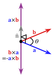
In the above picture, two vectors \(\vec{a}\) and \(\vec{b}\) are crossed to produce a 3rd vector \(\vec{c} = \vec{a}\times\vec{b}\). This vector \(\vec{c}\) is orthogonal to the vectors \(\vec{a}\) and \(\vec{b}\), meaning that \(\vec{c}\cdot\vec{a} = 0\) and \(\vec{c}\cdot\vec{b} = 0\). This is important for this next neat trick. Imagine we have points \(P_1\) and \(P_2\). To tie back into the example above, let's let \(\vec{a} = P_1 = (x_1,y_1,w_1)\) and \(\vec{b} = P_2 = (x_2,y_2,w_2)\). If we cross these vectors, we get a vector \(\vec{c} = \vec{a} \times\vec{b}\) for which \(\vec{c}\cdot\vec{a} = 0\) and \(\vec{c}\cdot\vec{b} = 0\). Since \(\vec{a}\) and \(\vec{b}\) are points, we could say that \(\vec{c} = (a,b,c)\), an implicit ordered triple that passes through both points. We can check that the line given by \((a,b,c)\) passes through both points by the dot product method. \[L(a,b,c) = P(X_1,Y_1,W_1) \times P(X_2,Y_2,W_2)\]
Line-Line Intersection
Using the same kind of logic, we can get the point at which 2 lines intersect. To use the cross product example again, let's let the vectors be the ordered triples of 2 implicit lines, \(\vec{a} = (a_1,b_1,c_1)\) and \(\vec{b} = (a_2,b_2,c_2)\). Again, crossing these vectors yields a vector \(\vec{c} = \vec{a} \times\vec{b}\) for which \(\vec{c}\cdot\vec{a} = 0\) and \(\vec{c}\cdot\vec{b} = 0\). Since \(\vec{a}\) and \(\vec{b}\) are lines, we could say that \(\vec{c} = (X,Y,W)\), the intersection point of both lines. This point has to be on both lines, and we can verify that using the dot-product method.
\[P(X,Y,W) = L(a_1,b_1,c_1) \times L(a_2,b_2,c_2)\]
Connection to Bezout's Theorem
Lines are degree-1 algebraic curves. Bezout's theorem states that 2 lines must intersect at exactly 1 point. So what happens with parallel lines? Well, if we use homogeneous coordinates, the intersection point will take the form \((X,Y,0)\), a point at infinity. Bezout's theorem still holds for that case.
Coding Tip: Any decent vector library will have a cross product method for 3D vectors (if not, coding one up is trivial). Passing in the ordered triples as vectors to the cross product function will return a 3D vector. This is the point in homogeneous form. In pseudocode:
Vector P = cross(new Vector(a1,b1,c1), new Vector(a2,b2,c2)); // check to see if the lines are parallel
if(P[2] != 0) { // this is to transform back to (x,y) from (X,Y,W)
	x = P[0] / P[2];
	y = P[1] / P[2];
}
Parametric-Implicit Curve Intersection
Sometimes it's advantageous to define some curves as parametric and some as implicit to solve for intersections. Most times, it's better to define the simpler curve as parametric and the more complex curve as implicit, if possible. This method solves for all algebraic intersections, which may or may not be "real" intersections.
Line-Circle Intersection
There are cases where there might be multiple roots, in which case we have to reconcile this with our intersection counting methods above (i.e. we have to count some of them differently). Let's take a fairly common case: line-circle intersection. Bezout's theorem says we will get 2 intersections since a circle is a degree-2 algebraic curve. The parametric line at point \((x_0,y_0)\) with direction \((c,d)\) and implicit circle centered at \((a,b)\) with radius \(r\) are defined as follows: \[ \begin{aligned} C(x,y) &= (x-a)^2+(y-b)^2-r^2 = 0 \\ L(x(t),y(t)) &= \begin{cases} x &= x_0+ct \\ y&=y_0+dt \end{cases} \end{aligned}\] We can substitute the parametric equations into the implicit equation to get a polynomial in terms of the parameter \(t\). The roots of the polynomial are the parameter values at which the line intersects the circle. Substituting, we get: \[ \begin{aligned} 0 &= (x_0+ct-a)^2+(y_0+dt-b)^2-r^2 \\ &= [c^2t^2+2c(x_0-a)t+(x_0-a)^2]+[d^2t^2+2d(y_0-b)t+(y_0-b)^2]-r^2 \\ &= (c^2+d^2)t^2+2[c(x_0-a)+d(y_0-b)]t + [(x_0-a)^2+(y_0-b)^2-r^2] \\ &= At^2+Bt+C \\ \end{aligned} \] This looks promising. The quadratic formula can solve really quickly for the roots of the polynomial: \[t=\frac{-B\pm\sqrt{B^2-4AC}}{2A}\] The result of this will either be 2 complex roots, 1 real root, or 2 real roots, depending on the discriminant \(B^2-4AC\). The 1 real root case means the line is tangent to the circle, which according to our intersection counting rules above, we count twice. (Note: technically we have 1 real root with multiplicity 2 since we have the roots \(t = (-B+0)/2A\) and \(t = (-B-0)/2A\).) Bezout's theorem still holds. That might be nice mathematically, but what does that mean for us? Well, the parameter \(t\) has to be a real number, so the real roots are values of \(t\) that the line intersects, so plugging the roots back into the parametric line gives us the Cartesian points of the intersection. What about the complex roots? Well, the restriction on \(t\) is that it has to be a real number, so in the case of 2 complex roots, we say the line doesn't intersect the circle.
Coding Tip: Here, it's easy enough to get the constants A, B, and C by following the formula. To check for intersections, just test if the discriminant \(B^2-4AC \ge 0\). If it's equal to zero, the line is tangent and the intersection point is just \(-B/2A\). Otherwise, use the quadratic formula to find the values of \(t\) and then plug them back into the parametric line equation to get the intersection points. In pseudocode:
A = c*c+d*d;
B = 2*(c(x0-a)+d(y0-b));
C = (x0-a)*(x0-a)+(y0-b)*(y0-b)-r*r;
disc = B*B-4*A*C;
if(disc == 0) {
   t = -B/(2*A);
   x1 = x0 + c*t;
   y1 = y0 + d*t;
   return [Point(x1,y1)];
} else if(disc > 0) {
   t1 = (-B+sqrt(disc))/(2*A);
   t2 = (-B-sqrt(disc))/(2*A);
   x1 = x0 + c*t1;
   y1 = y0 + d*t1;
   x2 = x0 + c*t2;
   y2 = y0 + d*t2;
   return [Point(x1,y1), Point(x2,y2)];
} else { return []; }
Line-Sphere Intersection
Line-sphere intersection is just like line-circle intersection. Algebraically, a sphere is also a degree-2 polynomial, and Bezout's theorem says we will still only get 2 intersections. The parametric line at point \((x_0,y_0,z_0)\) with direction \((p,q,r)\) and implicit sphere centered at \((a,b,c)\) with radius \(R\) are defined as follows: \[ \begin{aligned} S(x,y,z) &= (x-a)^2+(y-b)^2+(z-c)^2-R^2 = 0 \\ L(x(t),y(t),z(t)) &= \begin{cases} x &= x_0+pt \\ y&=y_0+qt \\ z&=z_0+rt \end{cases} \end{aligned}\] We can substitute the parametric equations into the implicit equation to get a polynomial in terms of the parameter \(t\). The roots of the polynomial are the parameter values at which the line intersects the circle. Substituting, we get: \[ \begin{aligned} 0 &= (x_0+pt-a)^2+(y_0+qt-b)^2+(z_0+rt-c)^2-R^2 \\ &= [p^2t^2+2p(x_0-a)t+(x_0-a)^2]+[q^2t^2+2q(y_0-b)t+(y_0-b)^2]+[r^2t^2+2r(z_0-c)t+(z_0-c)^2]-R^2 \\ &= (p^2+q^2+r^2)t^2+2[p(x_0-a)+q(y_0-b)+r(z_0-c)]t + [(x_0-a)^2+(y_0-b)^2+(z_0-c)^2-R^2] \\ &= At^2+Bt+C \\ \end{aligned} \] The solution method is exactly the same as for line-circle intersections.
Line-Plane Intersection
This is a simpler case than the line-circle intersection, although it involves a surface and a curve. A plane is algebraically a degree-1 polynomial in implicit form, so according to Bezout's theorem, they should intersect at exactly 1 point. We take the plane in implicit form and the line in parametric form and apply our method as above: \[ \begin{aligned} P(x,y) &= ax+by+cz+d=0 \\ L(x(t),y(t),z(t)) &= \begin{cases} x &= x_0+ut \\ y&=y_0+vt \\ z &= z_0+wt \\ \end{cases} \end{aligned}\] We substitute the parametric equations into the implicit form and solve for \(t\) as before:
\[ \begin{aligned} P(x(t),y(t),z(t)) = 0 &= a(x_0+ut)+b(y_0+vt)+c(z_0+wt)+d \\ &= (ax_0+by_0+cy_0+d) + (au+bv+cw)t \\ t &= -\frac{ax_0+by_0+cy_0+d}{au+bv+cw} \\ &= -\frac{(a,b,c,d)\cdot(x_0,y_0,z_0,1)}{(a,b,c,d)\cdot(u,v,w,0)} \end{aligned} \]
By substituting the value for \(t\) into the parametric line, we get the intersection point of the line and the plane. If the line runs parallel to the plane, the dot product of the plane normal and the line direction (which is the denominator) will be zero.
Coding Tip: Getting the plane and line into this form is probably the trickiest thing here. Once you've done that, you can use the dot product operation for a 4D vector to get what you're after (if your vector library doesn't support 4D dot product, either code it up or use the equation given above before the dot product representation). In pseudocode:
Vector4 PL = new Vector4(a,b,c,d);
Vector4 P = new Vector4(x0,y0,z0,1);
Vector4 D = new Vector4(u,v,w,0);
den = dot(PL,D);
if(den != 0) { // check for div by zero
	t = -dot(PL,P) / den;
	x = x0 + u*t;
	y = y0 + v*t;
	z = z0 + w*t;
}
Ray-Triangle Intersection One method of ray-triangle intersection is basically a two-step process, the first step being computing the point on the plane that intersects the ray (line). The next is to determine if the point lies inside the triangle. Barycentric coordinates is a common method of doing this, but another method would be to create lines in the plane with directions such that a point inside the triangle would be on the same side of each line (i.e. the point would be on the left or right sides of each line). The side of the line can be computed using the scaled signed distance as detailed above.
Higher-Degree Curve Intersection
Circle-Circle Intersection
This implicit-parametric curve intersection method can even work for higher degrees. Analytically, the Abel-Ruffini theorem states that there is no algebraic solution for a polynomial of degree 5 or higher, so beyond that we'll have to use numerical methods. In the case of circle-circle intersection, Bezout's theorem says we could get up to 4 intersections since a circle is a degree-2 algebraic curve, however only up to 2 of them will ever be real intersections. The parametric circle at point \((x_1,y_1)\) with radius \(r_1\) and implicit circle centered at \((x_0,y_0)\) with radius \(r_0\) are defined as follows:
\[ \begin{aligned} C(x,y) &= (x-x_0)^2+(y-y_0)^2-r_0^2 = 0 \\ L(x(t),y(t)) &= \begin{cases} x &= x_1+r_1 \cos{t} \\ y &= y_1+r_1 \sin{t} \end{cases} \end{aligned}\]
We can combine the equations as before:
\[ \begin{aligned} 0 &= (x_1+r_1 \cos{t} - x_0)^2+(y_1+r_1 \sin{t}-y_0)^2-r_0^2 \\ &= [(x_1-x_0)+r_1 \cos{t}]^2 + [(y_1-y_0)+r_1 \sin{t}]^2 - r_0^2 \\ &= [(x_1-x_0)^2 + 2 r_1 \cos{t}(x_1-x_0)+r_1^2 \cos{t}^2] + [(y_1-y_0)^2 + 2 r_1 \sin{t}(y_1-y_0)+r_1^2 \sin{t}^2] - r_0^2 \\ &= [(x_1-x_0)^2 + (y_1-y_0)^2] + 2 r_1 [\cos{t}(x_1-x_0)+\sin{t}(y_1-y_0)] + r_1^2 [\cos{t}^2 + \sin{t}^2] - r_0^2 \\ &= [(x_1-x_0)^2 + (y_1-y_0)^2 + (r_1^2- r_0^2)] + [2 r_1 (x_1-x_0)] \cos{t} + [2 r_1 (y_1-y_0)] \sin{t} \\ &= - c + a \cos{t} + b \sin{t} \\ \end{aligned} \]
Solving such a problem is a bit tricky, but we can try to take advantage of the sum angle identity because it has a similar structure: \[ \sin{(\alpha + \beta)} = \sin{\alpha}\cos{\beta}+\cos{\alpha}\sin{\beta} \] If we set \(t = \alpha\), we just have to find a \(\beta\) such that \(b = \cos{\beta}\) and \(a = \sin{\beta}\). There are two problems, however. Although \(\sin{\beta}^2 + \cos{\beta}^2 = 1\), we can't be sure that \(a^2+b^2=1\). As well, \(a\) and \(b\) have to be between -1 and 1 because that's the range of both the sine and cosine functions. If we alter the equation above to meet these criteria, we can apply the sum angle identity and solve. If we let \(A = \frac{a}{\sqrt{a^2+b^2}}\) and \(B = \frac{b}{\sqrt{a^2+b^2}}\), both coefficients are between -1 and 1 and \(A^2+B^2=1\). Thus we can set \(A = \sin{\beta}\) and \(B = \cos{\beta}\), and we can set up the following equation: \[ \begin{aligned} a \cos{t} + b \sin{t} &= \sqrt{a^2+b^2}(A \cos{t} + B \sin{t}) \\ &= \sqrt{a^2+b^2}(\sin{\beta} \cos{t} + \cos{\beta} \sin{t}) \\ &= \sqrt{a^2+b^2} \sin{(t +\beta)} \\ \end{aligned} \] Substituting into the top equation, we get \(\sqrt{a^2+b^2} \sin{(t +\beta)} = c\), or: \[\sin{(t +\beta)} = C\] where \(C = \frac{c}{\sqrt{a^2+b^2}}\). When solving this equation, remember although the arcsine function is one-to-one there are technically 2 values on the interval \([0,2\pi)\) that are solutions to the equation. With this we can solve the following with a few steps: Solve for \(\beta\) by using \(\tan{\beta} = A/B\). Solve for the 2 possible values of \(t+\beta) by using the last equation. Solve for possible values of t. Solve for the intersections by substituting the value of t into the parametric equation. Just like in the line-circle case, we can separate the 0, 1, and 2 intersection cases as follows: If \(|C| > 1 \) , then the circles don't intersect at all. If \(|C| = 1 \) , then the circles are tangent. If \(|C| < 1 \) , then the circles intersect in 2 places.
Advanced Intersections
Just to illustrate how general this method is, let's take a more advanced example: \[ \begin{aligned} C(x,y) &= x^2+y^2-1 = 0 \\ L(x(t),y(t)) &= \begin{cases} x &= 2t-1 \\ y&=8t^2-9t+1 \end{cases} \end{aligned}\]
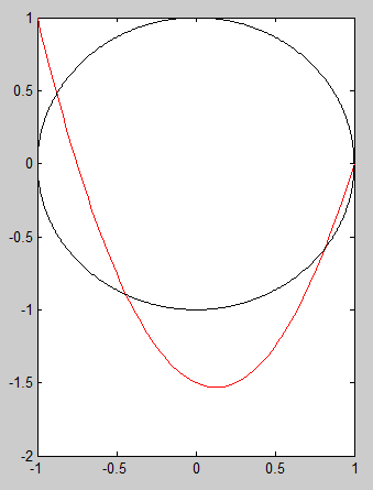
The picture above shows the curves. The red curve is the parametric curve and the black curve is the implicit curve. As you can see, there are 4 real intersections, and since both curves are degree-2 we should end up with all real roots. Inserting definitions of the parametric equations into the implicit form, we get: \[ \begin{aligned} f(x(t),y(t)) &= (2t-1)^2+(8t^2-9t+1)^2-1 \\ &= 64t^4-144t^3+101t^2-22t+1 \\ &= 0 \end{aligned} \] This is a quartic polynomial, so a more advanced numeric root finding method needs to be used, like bisection, regula falsi, or Newton's method. The roots of the polynomial are t = 0.06118, 0.28147, 0.90735, and 1.0. We do have all real roots, so Bezout's theorem is satisfied.
Higher-Degree Rational Curve Intersection
If the parametric curves are rational, then this method needs to be slightly modified. Rational parametric curves are usually of the form:
\[x = \frac{a(t)}{c(t)}, \, y = \frac{b(t)}{c(t)}\]
We can use homogeneous coordinates here really well. Since we have the mapping \((x,y) = (X/W,Y/W)\), we can define each homogeneous coordinate as \(X = a(t),\,Y = b(t),\,W=c(t)\). We also need to modify the implicit curve to handle homogeneous coordinates too, but this isn't very hard. Let's illustrate with an example:
\[ \begin{aligned} S(x,y) &= x^2+2x+y^2+1 = 0 \\ P(x(t),y(t)) &= \begin{cases} x &= \frac{t^2+t}{t^2+1} \\ y &= \frac{2t}{t^2+1} \\ \end{cases} \end{aligned}\]
Our parametric curve in homogeneous coordinates is \(X = t^2+t\),\(Y=2t\),and \(W={t^2+1}\). Our implicit curve can be changed to use homogeneous coordinates by substituting in the mapping \((x,y) = (X/W,Y/W)\): \[ \begin{aligned} S &= \left(\frac{X}{W}\right)^2+2\left(\frac{X}{W}\right)+\left(\frac{Y}{W}\right)^2+1 \\ &= X^2+2XW+Y^2+W^2 \\ \end{aligned} \] We can substitute our homogeneous coordinate equation into our modified implicit function:
\[ \begin{aligned} S &= (t^2+t)^2 + 2(t^2+t)(t^2+1) + (2t)^2 + (t^2+1)^2 \\ &= 4t^4+6t^3+5t^2+4t+1 \\ &= 0 \\ \end{aligned} \]
We get 2 real roots at t = 0.3576 and t = 1, and 2 complex roots. Both curves are degree-2, so we expect 4 intersections. We have 4 intersections total, so Bezout's theorem is satisfied. Parametric-Parametric Curve Intersection The way to solve intersections of 2 parametric curves is via implicitization of one of the curves. This can be a very fast method, but it suffers from numeric instability for high degree polynomials. We won't cover implicitization in this article, but there is a lot of literature on it out there.
Bezier Curve Intersection
A Bezier curve is just a degree-n Bernstein polynomial, which means it's just a regular polynomial of a different form. The above methods work well for Bezier curves, but they are more efficient and more numerically stable if modified slightly to take advantage of the Bernstein form. We won't cover this here, but there is literature out there on this as well.
Conclusion
These common methods of intersection testing can greatly aid any game programmer, whether purely for graphics or other game-specific logic. Hopefully you can make some use of these simple, yet powerful techniques. References A lot of the information here was taught to me by Dr. Thomas Sederberg (associate dean at Brigham Young University, inventor of the T-splines technology, and recipient of the 2006 ACM SIGGRAPH Computer Graphics Achievement Award). The rest came from my own study of relevant literature. The article image is from his self-published book, Computer-Aided Geometric Design.
Article Update Log
- 22 Apr 2017: Added a section for circle-circle intersection
- 23 Nov 2015: Added a motivating example to help those new to algebraic geometry
- 17 Nov 2015: Added a section for line-sphere intersection
- 03 Feb 2014: Added coding tips for applying the methods
- 15 Jan 2014: Initial release


I learned nothing from reading this.