Simulating physics can be fairly complex. Spatial motion (vehicles, projectiles, etc.), friction, collision, explosions, and other types of physical interactions are complicated enough to describe mathematically, but making them accurate when computed adds another layer on top of that. Making it run in real time adds even more complexity. There is lots of active research into quicker and more accurate methods. This article is meant to showcase a really interesting way to simulate particles with constraints in a numerically stable way. As well, I'll try to break down the underlying principles so it's more understandable by those who forgot their physics.
Note: the method presented in this article is described in the paper
"Interactive Dynamics" and was written by Witkin, Gleicher, and Welch. It was published in ACM in 1990.
A posted PDF of the paper can be found here:
http://www.cs.cmu.edu/~aw/pdf/interactive.pdf
A link to another article by Witkin on this subject can be found here:
https://www.cs.cmu.edu/~baraff/pbm/constraints.pdf
Physical Theory
Newton's Laws
Everyone's familiar with Newton's second law: \( F = ma\). It forms the basis of Newtonian mechanics. It looks very simple by itself, but usually it's very hard to deal with Newton's laws because of the number of equations involved. The number of ways a body can move in space is called the
degrees of freedom. For full 3D motion, we have 6 degrees of freedom for each body and thus need 6 equations per body to solve for the motion. For the ease in explaining this method, we will consider translations only, but this can be extended for rotations as well.
We need to devise an easy way to build and compute this system of equations. For a point mass moving in 3D, we can set up the general equations as a matrix equation:
\[ \left [ \begin{matrix} m_1 & 0 & 0 \\ 0 & m_1 & 0 \\ 0 & 0 & m_1 \\ \end{matrix} \right ] \left [ \begin{matrix} a_{1x} \\ a_{1y} \\ a_{1z} \\ \end{matrix} \right ] = \left [ \begin{matrix} F_{1x} \\ F_{1y} \\ F_{1z} \\ \end{matrix} \right ]\]
This can obviously be extended to include accelerations and net forces for many particles as well. The abbreviated equation is:
\[ M \ddot{q} = F \]
where \(M\) is the mass matrix, \(\ddot{q}\) is acceleration (the second time derivative of position), and \(F\) is the sum of all the forces on the body.
Motivating Example
One of the problems with computing with Newton-Euler methods is that we have to compute all the forces in the system to understand how the system will evolve, or in other words, how the bodies will move with respect to each other. Let's take a simple example of a pendulum.
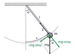
Technically, we have a force on the wall by the string, and a force on the ball by the string. In this case, we can reduce it to the forces shown and solve for the motion of the ball. Here, we have to figure out how the string is pulling on the ball ( \( T = mg \cos{\theta}\) ), and then break it into components to get the forces in each direction. This yields the following:
\[ \left [ \begin{matrix} m & 0 \\ 0 & m \\ \end{matrix} \right ] \left [ \begin{matrix} \ddot{q}_x \\ \ddot{q}_y \\ \end{matrix} \right ] = \left [ \begin{matrix} -T\sin{\theta} \\ -mg+T\cos{\theta} \\ \end{matrix} \right ]\]
We can then model this motion without needing to use the string. The ball can simply exist in space and move according to this equation of motion.
Constraints and Constraint Forces
One thing we've glossed over without highlighting in the pendulum example is the string. We were able to ignore the fact that the mass is attached to the string, so does the string actually do anything in this example? Well, yes and no. The string provides the tension to hold up the mass, but anything could do that. We could have had a rod or a beam hold it up. What it really does is define the possible paths the mass can travel on. The motion of the mass is dictated, or
constrained, by the string. Here, the mass is traveling on a circular path about the point where the pendulum hangs on the wall. Really, anything that constrains the mass to this path with no additional work can do this. If the mass was a bead on a frictionless circular wire with the same radius, we would get the same equations of motion!
If we rearrange the pendulum's equations of motion, we can illustrate a point:
\[ \left [ \begin{matrix} m & 0 \\ 0 & m \\ \end{matrix} \right ] \left [ \begin{matrix} \ddot{q}_x \\ \ddot{q}_y \\ \end{matrix} \right ] = \left [ \begin{matrix} 0 \\ -mg \\ \end{matrix} \right ] + \left [ \begin{matrix} -T\sin{\theta} \\ T\cos{\theta} \\ \end{matrix} \right ]\]
In our example, the only applied force on the mass is gravity. That is represented as the first term on the right hand side of the equation. So what's the second term? That is the
constraint force, or the other forces necessary to keep the mass constrained to the path. We can consider that a part of the net forces on the mass, so the modified equation is:
\[ M_{ij} \ddot{q}_j = Q_j + C_j \]
where \(M\) is the mass matrix, \(\ddot{q}\) is acceleration (the second time derivative of position), \(Q\) is the sum of all the
applied forces on the body, and \(C\) is the sum of all the constraint forces on the body. Let's note as well that the mass matrix is basically diagonal. It's definitely sparse, so that can work to our advantage later when we're working with it.
Principle of Virtual Work
The notion of adding constraint forces can be a bit unsettling because we are adding more forces to the body, which you would think would change the energy in the system. However, if we take a closer look at the pendulum example, we can see that the tension in the string is acting perpendicular (orthogonal) to the motion of the mass. If the constraint force is orthogonal to the displacement, then there is no additional work being done on the system, meaning no energy is being added to the system. This is called
d'Alembert's principle, or the principle of virtual work.
Believe it or not, this is a big deal! This is one of the key ideas in this method. Normally, springs are used to create the constraint forces to help define the motion between objects. For this pendulum example, we could treat the string as a very stiff spring. As the mass moves, it may displace a small amount from the circular path (due to numerical error). Then the spring force will move the mass back toward the constraint. As it does this, it may overshoot a little or a lot! In addition to this, sometimes the spring constants can be very high, creating what are aptly named
stiff equations. This causes the numerical integration to either take unnecessarily tiny time steps where normally larger ones would suffice. These problems are well-known in the simulation community and many techniques have been created to avoid making the equations of motion stiff.
As illustrated above, as long as the constraint forces don't do any work on the system, we can use them. There are lots of combinations of constraint forces that can be used that satisfy d'Alembert's principle, but we can illustrate a simple way to get those forces.
Witkin's Method
Constraints
Usually a simulation has a starting position \(q = \left [ \begin{matrix} x_1 & y_1 & z_1 & x_2 & y_2 & z_2 & \cdots \\ \end{matrix} \right ] \) and velocity \(\dot{q} = \left [ \begin{matrix} \dot{x}_1 & \dot{y}_1 & \dot{z}_1 & \dot{x}_2 & \dot{y}_2 & \dot{z}_2 & \cdots \\ \end{matrix} \right ] \). The general constraint function is based on the state \(q(t)\) and possibly on time as well: \(c(q(t))\). The constraints need to be implicit, meaning that the constraints should be an equation that equals zero. For example, the 2D implicit circle equation is \(x^2 + y^2 - R^2 = 0\).
Remember there are multiple constraints to take into consideration. The vector that stores them will be denoted in an index notation as \(c_i\). Taking the total derivative with respect to time is:
\[\dot{c}_i=\frac{d}{dt}c_i(q(t),t)=\frac{\partial c_i}{\partial q_j}\dot{q}_j+\frac{\partial c_i}{\partial t}\]
The first term in this equation is actually a matrix, the Jacobian of the constraint vector \(J = \partial c_i/\partial q_j\), left-multiplied to the velocity vector. The Jacobian is made of all the partial derivatives of the constraints. The second term is just the partial time derivative of the constraints.
Differentiating again to get \(\ddot{c_i}\) yields:
\[\ddot{c}_i = \frac{\partial c_i}{\partial q_j} \ddot{q}_j + \frac{\partial \dot{c}_i}{\partial q_j} \dot{q}_j + \frac{\partial^2 c_i}{\partial t^2}\]
Looking at the results, the first term is the Jacobian of the constraints multiplied by the acceleration vector. The second term is actually the Jacobian of the time derivative of the constraint. The third term is the second partial time derivative of the constraints.
The formulas for the complicated terms, like the Jacobians, can be calculated analytically ahead of time. As well, since the constraints are position constraints, the second time derivatives are accelerations.
Newton's Law with Constraints
If we solve the matrix Newton's Law equation for the accelerations, we get:
\[\ddot{q}_j = W_{jk}\left ( C_k + Q_k \right )\]
where \(W = M^{-1}\), the mass matrix inverse. If we were to replace this with the acceleration vector from our constraint equation, we would get the following:
\[\frac{\partial c_i}{\partial q_j} W_{jk}\left ( C_k + Q_k \right ) + \frac{\partial \dot{c}_i}{\partial q_j} \dot{q}_j + \frac{\partial^2 c_i}{\partial t^2} = 0\]
\[JW(C+Q) + \dot{J} \dot{q} + c_{tt} = 0\]
Here, the only unknowns are the constraint forces. From our discussion before, we know that the constraint forces must satisfy the principle of virtual work. As we said before, the forces need to be orthogonal to the displacements, or the legal paths. We will take the gradient of the constraint path to get vectors orthogonal to the path. The reason why this works will be explained later. Since the constraints are placed in a vector, the gradient of that vector would be the Jacobian matrix of the constraints: \(\partial c/\partial q\). Although the row vectors of the matrix have the proper directions to make the dot product with the displacements zero, they don't have the right magnitudes to force the masses to lie on the constraint. We can construct a vector of scalars that will multiply with the row vectors to make the magnitudes correct. These are known as
Lagrange multipliers. This would make the equation for the constraint forces as follows:
\[C_j = \lambda_i \frac{\partial c_i}{\partial q_j} = J^T \lambda_i\]
Plugging that equation back into the augmented equation for Newton's law:
\[ \left ( -JWJ^T \right ) \lambda = JWQ + \dot{J}\dot{q} + c_{tt}\]
Note that the only unknowns here are the Lagrange multipliers.
Attempt at an Explanation of the Constraint Force Equation
If you're confused at how Witkin got that equation for the constraint forces, that's normal. I'll attempt to relate it to something easier to visualize and understand: surfaces. Let's take a look at the equation of a quadric surface:
\[Ax^2+By^2+Cz^2+Dxy+Eyz+Fxz+Gx+Hy+Iz+J=0\]
The capital letters denote constants. Notice also the equation is implicit. We can see the equation for an ellipse is a quadric surface:
\[f(x,y,z) = (1/a^2)x^2+(1/b^2)y^2+(1/c^2)z^2-1=0\]
For a point (x,y,z) to be on the surface, it must satisfy this equation. To put it into more formal math terms, we could say the surface takes a point in \(\mathbb{R}^3\) and maps it to the zero vector in \(\mathbb{R}\), which is just 0. Any movement on this surface is "legal" because the new point will still satisfy the surface equation. If we were to take the gradient of this ellipse equation, we'd get:
\[ \left [ \begin{matrix} \frac{\partial f}{\partial x} \\ \frac{\partial f}{\partial y} \\ \frac{\partial f}{\partial z} \\ \end{matrix} \right ] = \left [ \begin{matrix} \frac{2x}{a^2} \\ \frac{2y}{b^2} \\ \frac{2z}{c^2} \\ \end{matrix} \right ] \]
This vector is the normal to the surface at the given (x,y,z) coordinates. If we were to visualize a plane tangent to the ellipse at that point, the dot product of the normal and the tangent plane would be zero by definition.
With this same type of thinking, we can see the constraints as a type of algebraic surface since they're also implicit equations (it's hard to visualize these surfaces geometrically since they can be n-dimensional). Just like with the geometry example, if we were to take the gradient of the constraints the resulting vector would be orthogonal to a tangent plane on the surface. In more formal math terms, the constraints/surfaces can be called the
null space since it contains all the points (vectors) that map to the zero vector. The gradients/normals to these constraints is termed the
null space complement. The constraint force equation produces vectors that lie in the null space complement, and are therefore orthogonal to the constraint surface.
The purpose of these math terms are to help generalize this concept for use in situations where the problems are not easy to visualize or intuitively understand.
Calculating the State
With these equations in place, the process of calculating the system state can now be summed up as follows:
- Construct the \(W\), \(J\), \(\dot{J}\), \(c_{tt}\) matrices.
- Multiply and solve the \(Ax=b\) problem for the Lagrange multipliers \(\lambda\).
- Compute the constraint forces using \(C = J^T \lambda\).
- Compute the accelerations using \(\ddot{q} = W(C+Q)\).
- Integrate the accelerations to get the new velocities \( \dot{q}(t) \) and positions \( q(t) \).
This process can be optimized to take advantage of sparsity in the matrices. The Jacobian matrix wll generally be sparse since the constraints won't generally depend on a large number of particles. This can help with the matrix multiplication on both sides. The main challenge will be in building these matrices.
Feedback
Due to numerical error, there will be a tendency to drift away from the proper solution. Recall that in order to derive the modified Newton's law equation above, we forced \( c_i = 0 \) and \( \dot{c_i} = 0 \). Numerical error can produce solutions that won't satisfy these equations within a certain tolerance, so we can use a method used in control systems engineering: the PID loop.
In most systems we want to control, there are inputs to the system (force, etc.) and measurements of a system's state (angle, position, etc.). A PID loop feeds the error in the actual and desired state back into the force inputs to drive the error to zero. For example, the human body has many different inputs to the force on the muscles when we stand upright. The brain measures many different things to see if we're centered on our feet or if we're teetering to one side or another. If we're falling or we're off-center, the brain makes adjustments to our muscles to stay upright. A PID loop does something similar by measuring the error and feeding that back into the inputs. If done correctly, the PID system will drive the error in the measured state to zero by changing the inputs to the system as needed.
Here, we use the error in the constraint and the constraint derivative to feedback into the system to better control the numerical drift. We augment the forces by adding terms that account for the \(c_i =0\) and \(\dot{c_i}=0\):
\[ F_j = Q_j + C_j + \alpha c_i \frac{\partial c_i}{\partial q_j} + \beta \dot{c_i} \frac{\partial c_i}{\partial q_j} \]
This isn't a true force being added since these extra terms will vanish when the forces are correct. This is just to inhibit numerical drift, so the constants \(\alpha\) and \(\beta\) are "magic", meaning that they are determined empirically to see what "fits" better.
Conclusion
Witkin's method for interactive simulations is pretty widely applicable. Although this can be obviously used for movable truss structures and models of Tinkertoys, he also talks about using them for deformable bodies, non-linear optimization and keyframe animation as well. There are lots of applications of this method. Hopefully this showcase of Witkin's method will help make this interesting solution more accessible to anyone doing any type of simulation engines.
Article Update Log
27 Aug 2015: Initial release


wish more articles came to me as well formatted as this one :) Other than a few minor grammatical corrections, I got stuck on this:
Second paragraph in Calculating the State