Original Post: Limitless Curiosity

Out of various phases of the physics engine. Constraint Resolution was the hardest for me to understand personally. I need to read a lot of different papers and articles to fully understand how constraint resolution works. So I decided to write this article to help me understand it more easily in the future if, for example, I forget how this works.

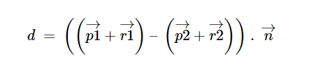
This article will tackle this problem by giving an example then make a general formula out of it. So let us delve into a pretty common scenario when two of our rigid bodies collide and penetrate each other as depicted below.

From the scenario above we can formulate:

We don't want our rigid bodies to intersect each other, thus we construct a constraint where the penetration depth must be more than zero.

\(C: d>=0\)

This is an inequality constraint, we can transform it to a more simple equality constraint by only solving it if two bodies are penetrating each other. If two rigid bodies don't collide with each other, we don't need any constraint resolution. So:

if d>=0, do nothing else if d < 0 solve C: d = 0

Now we can solve this equation by calculating  \( \Delta \vec{p1},\Delta \vec{p2},\Delta \vec{r1}\),and  \( \Delta \vec{r2}\)  that cause the constraint above satisfied. This method is called the position-based method. This will satisfy the above constraint immediately in the current frame and might cause a jittery effect.

A much more modern and preferable method that is used in Box2d, Chipmunk, Bullet and my physics engine is called the impulse-based method. In this method, we derive a velocity constraint equation from the position constraint equation above.

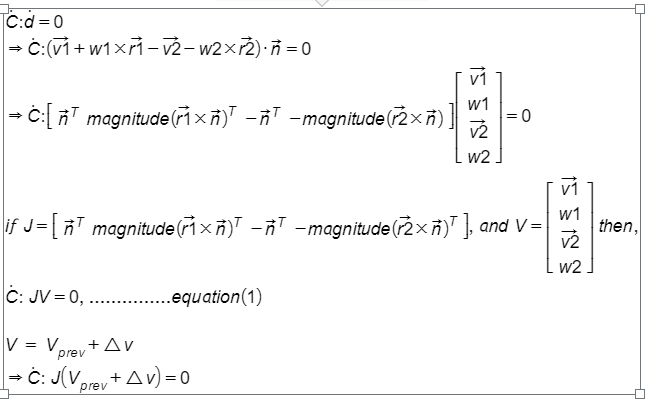
We are working in 2D so angular velocity and the cross result of two vectors are scalars.

Next, we need to find \(\Delta V\) or impulse to satisfy the velocity constraint. This \(\Delta V\) is caused by a force. We call this force 'constraint force'. Constraint force only exerts a force on the direction of illegal movement in our case the penetration normal. We don't want this force to do any work, contribute or restrict any motion of legal direction.

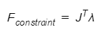
\(\lambda\) is a scalar, called Lagrangian multiplier. To understand why constraint force working on \(J^{T}\) direction (remember J is a 12 by 1 matrix, so \(J^{T}\) is a 1 by 12 matrix or a 12-dimensional vector), try to remember the equation for a three-dimensional plane.

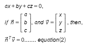
Now we can draw similarity between equation(1) and equation(2), where \(\vec{n}^{T}\) is similar to J and \(\vec{v}\) is similar to V. So we can interpret equation(1) as a 12 dimensional plane, we can conclude that \(J^{T}\) as the normal of this plane. If a point is outside a plane, the shortest distance from this point to the surface is the normal direction.

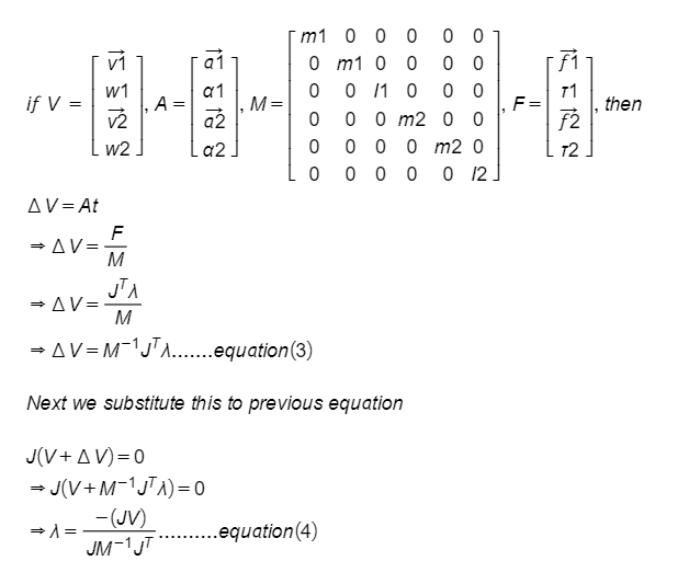
After we calculate the Lagrangian multiplier, we have a way to get back the impulse from equation(3). Then, we can apply this impulse to each rigid body.

Baumgarte Stabilization

Note that solving the velocity constraint doesn't mean that we satisfy the position constraint. When we solve the velocity constraint, there is already a violation in the position constraint. We call this violation position drift. What we achieve is stopping the two bodies from penetrating deeper (The penetration depth will stop growing). It might be fine for a slow-moving object as the position drift is not noticeable, but it will be a problem as the object moving faster. The animation below demonstrates what happens when we solve the velocity constraint.

[caption id="attachment_38" align="alignnone" width="800"]

So instead of purely solving the velocity constraint, we add a bias term to fix any violation that happens in position constraint. 

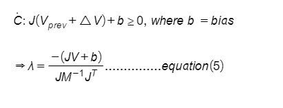
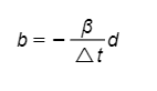
So what is the value of the bias? As mentioned before we need this bias to fix positional drift. So we want this bias to be in proportion to penetration depth.

This method is called Baumgarte Stabilization and \(\beta\) is a baumgarte term. The right value for this term might differ for different scenarios. We need to tweak this value between 0 and 1 to find the right value that makes our simulation stable.

Sequential Impulse

If our world consists only of two rigid bodies and one contact constraint. Then the above method will work decently. But in most games, there are more than two rigid bodies. One body can collide and penetrate with two or more bodies. We need to satisfy all the contact constraint simultaneously. For a real-time application, solving all these constraints simultaneously is not feasible. Erin Catto proposes a practical solution, called sequential impulse. The idea here is similar to Project Gauss-Seidel. We calculate \(\lambda\) and \(\Delta V\) for each constraint one by one, from constraint one to constraint n(n = number of constraint). After we finish iterating through the constraints and calculate \(\Delta V\), we repeat the process from constraint one to constraint n until the specified number of iteration. This algorithm will converge to the actual solution.The more we repeat the process, the more accurate the result will be. In Box2d, Erin Catto set ten as the default for the number of iteration.

Another thing to notice is that while we satisfy one constraint we might unintentionally satisfy another constraint. Say for example that we have two different contact constraint on the same rigid body.

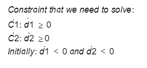
When we solve \(\dot{C1}\), we might incidentally make \(\dot{d2} >= 0\). Remember that equation(5), is a formula for \(\dot{C}: \dot{d} = 0\) not \(\dot{C}: \dot{d} >= 0\). So we don't need to apply it to \(\dot{C2}\) anymore. We can detect this by looking at the sign of \(\lambda\). If the sign of \(\lambda\) is negative, that means the constraint is already satisfied. If we use this negative lambda as an impulse, it means we pull it closer instead of pushing it apart. It is fine for individual \(\lambda\) to be negative. But, we need to make sure the accumulation of \(\lambda\) is not negative. In each iteration, we add the current lambda to normalImpulseSum. Then we clamp the normalImpulseSum between 0 and positive infinity. The actual Lagrangian multiplier that we will use to calculate the impulse is the difference between the new normalImpulseSum and the previous normalImpulseSum

Restitution

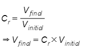
Okay, now we have successfully resolve contact penetration in our physics engine. But what about simulating objects that bounce when a collision happens. The property to bounce when a collision happens is called restitution. The coefficient of restitution denoted \(C_{r}\), is the ratio of the parting speed after the collision and the closing speed before the collision.

The coefficient of restitution only affects the velocity along the normal direction. So we need to do the dot operation with the normal vector.

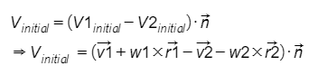
Notice that in this specific case the \(V_{initial}\) is similar to JV. If we look back at our constraint above, we set \(\dot{d}\) to zero because we assume that the object does not bounce back(\(C_{r}=0\)).So, if \(C_{r} != 0\), instead of 0, we can modify our constraint so the desired velocity is \(V_{final}\).

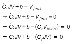
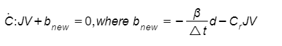
We can merge our old bias term with the restitution term to get a new bias value.

// init constraint
// Calculate J(M^-1)(J^T). This term is constant so we can calculate this first
for (int i = 0; i < constraint->numContactPoint; i++)
{
  ftContactPointConstraint *pointConstraint = &constraint->pointConstraint;

  pointConstraint->r1 = manifold->contactPoints.r1 - (bodyA->transform.center + bodyA->centerOfMass);
  pointConstraint->r2 = manifold->contactPoints.r2 - (bodyB->transform.center + bodyB->centerOfMass);

  real kNormal = bodyA->inverseMass + bodyB->inverseMass;

  // Calculate r X normal
  real rnA = pointConstraint->r1.cross(constraint->normal);
  real rnB = pointConstraint->r2.cross(constraint->normal);

  // Calculate J(M^-1)(J^T).
  kNormal += (bodyA->inverseMoment * rnA * rnA + bodyB->inverseMoment * rnB * rnB);

  // Save inverse of J(M^-1)(J^T).
  pointConstraint->normalMass = 1 / kNormal;

  pointConstraint->positionBias = m_option.baumgarteCoef *

  manifold->penetrationDepth;
  ftVector2 vA = bodyA->velocity;
  ftVector2 vB = bodyB->velocity;
  real wA = bodyA->angularVelocity;
  real wB = bodyB->angularVelocity;
  ftVector2 dv = (vB + pointConstraint->r2.invCross(wB) - vA - pointConstraint->r1.invCross(wA));
  //Calculate JV
  real jnV = dv.dot(constraint->normal
  pointConstraint->restitutionBias = -restitution * (jnV + m_option.restitutionSlop);
 }

// solve constraint
while (numIteration > 0)
{

  for (int i = 0; i < m_constraintGroup.nConstraint; ++i) { 
    ftContactConstraint *constraint = &(m_constraintGroup.constraints); int32 bodyIDA = constraint->bodyIDA;
    int32 bodyIDB = constraint->bodyIDB;
    ftVector2 normal = constraint->normal;
    ftVector2 tangent = normal.tangent();

    for (int j = 0; j < constraint->numContactPoint; ++j)
    {
      ftContactPointConstraint *pointConstraint = &(constraint->pointConstraint[j]);

      ftVector2 vA = m_constraintGroup.velocities[bodyIDA];
      ftVector2 vB = m_constraintGroup.velocities[bodyIDB];
      real wA = m_constraintGroup.angularVelocities[bodyIDA];
      real wB = m_constraintGroup.angularVelocities[bodyIDB];

      //Calculate JV. (jnV = JV, dv = derivative of d, JV = derivative(d) dot normal))
      ftVector2 dv = (vB + pointConstraint->r2.invCross(wB) - vA - pointConstraint->r1.invCross(wA));
      real jnV = dv.dot(normal);

      //Calculate Lambda ( lambda
      real nLambda = (-jnV + pointConstraint->positionBias / dt + pointConstraint->restitutionBias) *
      pointConstraint->normalMass;

      // Add lambda to normalImpulse and clamp
      real oldAccumI = pointConstraint->nIAcc;
      pointConstraint->nIAcc += nLambda;
      if (pointConstraint->nIAcc < 0) { pointConstraint->nIAcc = 0;
      }
      // Find real lambda
      real I = pointConstraint->nIAcc - oldAccumI;

      // Calculate linear impulse
      ftVector2 nLinearI = normal * I;

      // Calculate angular impulse
      real rnA = pointConstraint->r1.cross(normal);
      real rnB = pointConstraint->r2.cross(normal);
      real nAngularIA = rnA * I;
      real nAngularIB = rnB * I;

      // Apply linear impulse
      m_constraintGroup.velocities[bodyIDA] -= constraint->invMassA * nLinearI;
      m_constraintGroup.velocities[bodyIDB] += constraint->invMassB * nLinearI;

      // Apply angular impulse
      m_constraintGroup.angularVelocities[bodyIDA] -= constraint->invMomentA * nAngularIA;
      m_constraintGroup.angularVelocities[bodyIDB] += constraint->invMomentB * nAngularIB;
    }
  }
  --numIteration;
}

General Step to Solve Constraint

In this article, we have learned how to solve contact penetration by defining it as a constraint and solve it. But this framework is not only used to solve contact penetration. We can do many more cool things with constraints like for example implementing hinge joint, pulley, spring, etc.

So this is the step-by-step of constraint resolution:

1. Define the constraint in the form \(\dot{C}: JV + b = 0\). V is always \(\begin{bmatrix} \vec{v1} \\ w1 \\ \vec{v2} \\ w2\end{bmatrix}\) for every constraint. So we need to find J or the Jacobian Matrix for that specific constraint.
2. Decide the number of iteration for the sequential impulse.
3. Next find the Lagrangian multiplier by inserting velocity, mass, and the Jacobian Matrix into this equation:
4. Do step 3 for each constraint, and repeat the process as much as the number of iteration.
5. Clamp the Lagrangian multiplier if needed.

This marks the end of this article. Feel free to ask if something is still unclear. And please inform me if there are inaccuracies in my article. Thank you for reading.

NB: Box2d use sequential impulse, but does not use baumgarte stabilization anymore. It uses full NGS to resolve the position drift. Chipmunk still use baumgarte stabilization.

References

1. Allen Chou's post on Constraint Resolution
2. A Unified Framework for Rigid Body Dynamics
3. An Introduction to Physically Based Modeling: Constrained Dynamics
4. Erin Catto's Box2d and presentation on constraint resolution

Falton Debug Visualizer 18_01_2018 22_40_12.mp4

equation.svg