This article has since been revised and updated from its original published version you see here.
[size="5"]
Preface
Hey there! This tutorial is for those who are new to 3D programming, and need to brush up on that math. I will teach you two primary things here, Vectors and Matrices (with determinants). I'm not going to go into everything, so this isn't designed as a standalone reference. A lot of mathematics books can probably discuss this much better, but anyway, without further ado, lets get on with it shall we?
[size="5"]
Vectors
[size="3"]
Vector basics - What is a vector?
Vectors are the backbone of games. They are the foundation of graphics, physics modelling, and a number of other things. Vectors can be of any dimension, but are most commonly seen in 2 or 3 dimensions. I will focus on 2D and 3D vectors in this text. Vectors are derived from hyper-numbers, a sub-set of hyper-complex numbers. But enough of that, you just want to know how to use them right? Good.
The notation for a vector is that of a bold lower-case letter, like
i, or an italic letter with an underscore, like
i. I'll use the former in this text. You can write vectors in a number of ways, and I will teach you 2 of them:
vector equations and
column vectors. Vectors can also be written using the two end points with an arrow above them. So, if you have a vector between the two points A and B, you can write that as

.
A vector equation takes the form
a= xi +
yj +
zk
i,
j and
k are unit vectors in the 3 standard Cartesian directions.
i is a unit vector aligned with the x axis,
j is a unit vector aligned with the y axis, and
k is a unit vector aligned with the z axis. Unit vectors are discussed later.
The coefficients of the
i,
j and
k parts of the equation are the vector's
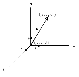
components. These are how long each vector is in each of the 3 axes. This may be easier to understand with the aid of a diagram.

This diagram shows a vector from the origin to the point ( 3, 2, 5 ) in 3D space. The
components of this vector are the
i,
j and
k coefficients ( 2, 3 and 5 ). So, in the above example, the vector equation would be:
a = 2
i + 3
j + 5
k
This can also be related to the deltas of a line going through 2 points.
The second way of writing vectors is as
column vectors. These are written in the following form

where
x,
y and
z are the components of that vector in the respective directions. These are exactly the same as the components of the vector equation. So in column vector form, the above example could be written as:

There are various advantages to both of the above forms, but I will continue to use the column vector form, as it is easier when it comes to matrices.
Position vectors are those that originate from the origin. These can define points in space, relative to the origin.
[size="3"]
Vector Math
You can manipulate vectors in various ways, including scalar multiplication, addition, scalar product and vector product. The latter two are extremely useful in 3D applications.
There are a few things you should know before moving to the methods above. The first is finding the
modulus (also called the
magnitude) of a vector. This is basically its length. This can be easily found using Pythagorean theorem, using the vector components. The modulus of
a is written |
a|.

in 3D and

in 2D, where
x,
y and
z are the components of the vector in the 3 axes of movement.
Unit vectors are vectors with a magnitude of 1, so |
a| = 1.
Addition
Vector addition is pretty easy. All you do is add the respective components together. So for instance, take the vectors:


The addition of these vectors would be:

Get it? This can also be represented very easily in a diagram, but I will only consider this in 2D, because it's easier to draw.


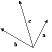
This works in the same way as moving the second vector so that its beginning is at the first vector's end, and taking the vector from the beginning of the first vector to the end of the second one. So, in a diagram, using the above example, this would be:

This means that you can add multiple vectors together to get the
resultant vector. This is used extensively in mechanics for finding resultant forces.
Subtracting
Subtracting is very similar to adding, and is also quite helpful. All you do is subtract the components in one vector from the components in the other. The geometric representation however is very different.
Let

and

Then

The visual representation of this is:
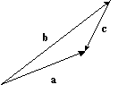
Here,
a and
b are set to be from the same origin. The vector
c is the vector from the end of the second vector to the end of the first, which in this case is from the end of
b to the end of
a. It may be easier to think of this as a vector addition.
Where instead of having:
c =
a -
b
we have
c = -
b +
a
which, according to what was said about the addition of vectors would produce:
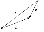
You can see that putting
a on the end of -
b has the same result.
Scalar multiplication
Scalar multiplication is easy to come to grips with. All you do is multiply each component by that scalar.
So, say you had the vector
a and a scalar
k, you would multiply each component by the scalar, getting this result:


This has the effect of lengthening or shortening the vector by the amount
k. For instance, take
k = 2; this would make the vector
a twice as long. Multiplying by a negative scalar reverses the direction of the vector. You can use scalar multiplication to find the unit vector of another vector. So, take the following example:

To find the unit vector of this, we would divide
a by |
a|. Calling the unit vector "
b":

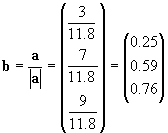
That is the unit vector
b in the direction of
a. This just scales each of the components, so that the magnitude is equal to 1.
Scalar multiplication is also used in the vector equation discussed earlier. The constants
x,
y and
z are the scalars that scale the
i,
j and
k vectors, before adding them to find the resultant vector.
The Scalar Product (Dot Product)
The
scalar product, also known as the
dot product, is very useful in 3D graphics applications. The scalar product is written

and is read "
a dot
b".
The definition the scalar product is the following:

Where q is the angle between the 2 vectors
a and
b. This produces a scalar result, hence the name scalar product. From this you can see that the scalar product of 2 parallel unit vectors is 1, as |
a||
b| = 1, and cos(0) also is 1. You should also have seen that the scalar product of two perpendicular vectors is 0, as cos(90) = 0, which makes the rest of the expression 0. The geometric interpretation is:

The scalar product can also be written in terms of Cartesian components., I will not go into how this is derived, but the final, simplified formula of
a.
b is:


We can now put these two equations equal to each other, yielding the equation:

With this, we can find angles between vectors. This is used extensively in the lighting part of the graphics pipeline, as it can see whether a polygon is facing towards or away from the light source. This is also used in deciding what side of planes points are on, which is also used extensively for culling.
The Vector Product (Cross Product)
The
vector product, which is also commonly known as the
cross product is also useful. The vector product basically finds a vector perpendicular to two other vectors. Great for finding normal vectors to surfaces.
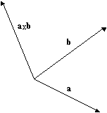
For those that are already familiar with determinants, the vector product is basically the expansion of the following determinant:

For those that aren't, the vector product in expanded form is:

Read "
a cross
b".
Since the cross product finds the perpendicular vector, we can say that:
i x
j =
k
j x
k =
i
k x
i =
j
Using scalar multiplication along with the vector product we can find the "normal" vector to a plane. A plane can be defined by two vectors,
a and
b. The normal vector is a vector that is perpendicular to a plane and is also a unit vector. Using the formulas discussed earlier, we have:


This first finds the vector perpendicular to the plane made by
a and
b then scales that vector so it has a magnitude of 1. Note however, that there are 2 possible normals to the plane defined by
a and
b. You will get different results by swapping
a and
b in the vector product. That is:

This is a very important point. If you put the inputs the wrong way round, the graphics API will not produce the desired lighting, as the normal will be facing in the opposite direction.
The Vector Equation of a Straight Line
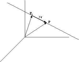
The vector equation of a straight line is very useful, and is given by a point on the line and a vector parallel to it:

Where
p[sub]0[/sub] is a point on the line and
v is the vector.
t is called the parameter, and scales
v. From this it is easy to see that as
t varies, a line is formed in the direction of
v. If
t only takes positive values, then
p[sub]0[/sub] is the starting point of the line. Diagrammatically, this is:
In expanded form, the equation becomes:


This is called the
parametric form of a straight line.
Using this to find the vector equation of a line through two points is easy:

If
t is confined to values between 0 and 1, then what you have is a
line segment between the points
p[sub]0[/sub] and
p[sub]1[/sub].
Using the vector equation we can define planes, and test for intersections. I won't go into planes much here, as there are many tutorials on them elsewhere, I'll just skim over it.
A plane can be defined as a point on the plane, and two vectors that are parallel to the plane, or:

where
s and
t the parameters and
u and
v are the vectors that are parallel to the plane. Using this, it becomes easy to find the intersection of a line and a plane, because the point of intersection must lie on both the line and the plane, so we simply make the two equations equal to each other.
Take the line:

and the plane:

To find the intersection point we simply equate, so that:

Ed. note: The
v on the left in the above equation is not the same vector as the
v on the right.
We then solve for
w,
s and
t, and then plug into either the line or plane equation to find the point. When testing for a line segment intersection,
w must be between 0 and 1.
There are many benefits for using the normal-distance form of a plane too. It's especially useful for testing what sides of a plane points or other shaped objects are. To do this, you dot the normal vector and the position vector of the point being tested, and add the distance of the plane from the origin.
So, if you have the plane

and the point
( x, y, z ), the point is in front of the plane if

and behind if it is < 0. If the result equals zero, the point is on the plane. This is used heavily in culling and BSP trees.
[size="5"]
Matrices
[size="3"]
What is a Matrix anyway?
A matrix can be considered a 2D array of numbers. They take the form:

Matrices are very powerful, and form the basis of all modern computer graphics, the advantage of them being that they are so fast. We define a matrix with an upper-case bold type letter. Look at the above example. The dimension of a matrix is its height followed by its width, so the above example has dimension 3x3. Matrices can be of any dimensions, but in terms of computer graphics, they are usually kept to 3x3 or 4x4. There are a few types of special matrices; these are the
column matrix,
row matrix,
square matrix,
identity matrix and
zero matrix. A column matrix is one that has a width of 1, and a height of greater than 1. A row matrix is a matrix that has a width of greater than 1, and a height of 1. A square matrix is when the dimensions are the same. For instance, the above example is a square matrix, because the width equals the height. The identity matrix is a special type of matrix that has values in the diagonal from top left to bottom right as 1 and the rest as 0. The identity matrix is known by the letter [font="Times New Roman"]
I[/font], where

The identity matrix can be any dimension, as long as it is also a square matrix. The zero matrix is a matrix that has all its elements set to 0.
The
elements of a matrix are all the numbers in it. They are numbered by the row/column position so that :

Vectors can also be used in column or row matrices. I will use column matrices here so that it is easier to understand. A 3D vector
a in matrix form will use a matrix
A with dimension 3x1 so that:

which you can see is the same layout as using column vectors.
[size="3"]
Matrix arithmetic
I won't go into every matrix manipulation, but instead I'll focus on the ones that are used extensively in computer graphics.
Matrix Multiplication
There are two ways to multiply a matrix: by a scalar, and by another conformable matrix. First, let's deal with the matrix/scalar multiplication.
This is pretty easy, all you do is multiply each element by the scalar. So, let
A be the original matrix,
B be the matrix after multiplication, and
k the constant. We perform:

where
i and
j are the positions in the matrix.
this can also be written as:

Multiplying a matrix by another matrix is more difficult. First, we need to know if the two matrices are
conformable. For a matrix to be conformable with another matrix, the number of rows in
A needs to equal the number of columns in
B. For instance, take matrix
A as having dimension 3x3 and matrix
B having dimension 3x2. These two matrices are conformable because the number of rows in
A is the same as the number of columns in
B. This is important as you'll see later. The product of these two matrices is another matrix with dimension 3x2. So, in general terms:
Take three matrices
A,
B and
C where
C is the product of
A and
B.
A and
B have dimension
mx
n and
px
q respectively. They are conformable if
n=p. The matrix
C has dimension
mx
q.
You perform the multiplication by multiplying each row in
A by each column in
B. So let
A have dimension 3x3 and
B have dimension 3x2.


So, with that in mind, let's try an example:


It's as simple as that! Some things to note:

A matrix multiplied by the identity matrix is the same, so:

The
transpose of a matrix is it flipped on the diagonal from the top left to the bottom right, so for example:

The transpose of this matrix would be:

Simple enough eh? And you thought it was going to be hard!
[size="3"]
Determinants
I'm going to talk a little bit about determinants now, as they are useful for solving certain types of equations. I will discuss easy 2x2 determinants first.
Take a 2x2 matrix:

The determinant of a matrix
A is written |
A| and is:

For higher dimension matrices, the determinant gets more complicated. Let's discuss a 3x3 matrix. You pass along the first row, and at each element, you discount the row and column that intersects it, and calculate the determinant of the resultant 2x2 matrix multiplied by that value.
So, for example, take this 3x3 matrix:

Ok then, Step 1: move to the first value in the top row,
a[sub]11[/sub] . Take out the row and column that intersects with that value. Step 2: multiply that determinant by
a[sub]11[/sub]. So, using diagrams:
Step1:

Step2:

We repeat this all along the top row, with the sign in front of the value of the top row alternating between a "+" and a "-", so the determinant of
A would be:

Now, how do we use these for equation solving? Good question. I will first show you how to solve a pair of equations with 2 unknowns.
Take the two equations:

We first
push the coefficients of the variables into a determinant, producing:

You can see it's laid out in the same way, which makes it easy. Now, to solve the equation in terms of
x, we replace the x coefficients in the determinant with the constants
k[sub]1[/sub] and
k[sub]2[/sub], dividing the result by the original determinant. So, that would be:

To solve for
y we replace the y coefficients with the constants instead.
Let's try an example to see this working:

We push the coefficients into a determinant, and solve:

To find
x substitute constants into
x co-efficients, and divide by
D:

To find
y substitute constants into
y co-efficients and divide by
D:

See, it's as simple as that! Just for good measure, I'll do an example using 3 unknowns in 3 equations:


Solve for
x:

Solve for
y:

Solve for
z:

And there we have it, how to solve a series of simultaneous equations using determinants, something that can be very useful.
Matrix Inversion
Equations can also be solved by inverting a matrix. Take the following equations again:

We push these into 3 matrices to solve:

Let's give these names such that:

We need to solve for B, and since there is no "matrix divide" operation, we need to invert the matrix
A and multiply it by
D, such that:

Now we need to know how to actually do the matrix inversion. There are many ways to do this, and the way I am going to show you is by no means the fastest.
To find the inverse of a matrix, we need to first find its
co-factor. We use a method similar to what we used when finding the determinant. What you do is this: at every element, eliminate the row and column that intersects it, and make it equal the determinant of the remaining part of the matrix. Let's find the first element in a 3x3 matrix. Let's call it c[sub]11[/sub]. We need to get rid of the row and column that intersects this, so that:

c[sub]11[/sub] will then take the value of the following determinant:

The sign in front of c[sub]11[/sub] is decided by the expression:

Where
i and
j are the positions of the element in the matrix.
That's easy enough isn't it? Thought so J. Just do the same for every element, and build up the co-factor matrix. Done? Good. Now that the co-factor matrix has been found, the inverse matrix can be calculated using the following equation:

Taking the previous example and equations, let's find the inverse matrix of
A.
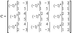
First, the co-factor matrix
C would be:

and |
A| is:

So
A--[sup]-1[/sup] is:

To solve the equations, we then do:


We can then find the values of
x,
y and
z by pulling them out of the last matrix, such that x = -62, y = 39 and z = 3, which is what the other method using determinants found.
A matrix is called
orthogonal if its inverse equals its transpose.
[size="3"]
Matrices in computer graphics
All graphics APIs use a set of matrices to define transformations in space. A transformation is a change, be it translation, rotation, or whatever. Using column a matrix to define a point in space, a
vertex, we can define matrices that alter that point in some way.
Transformation Matrices
Most graphics APIs use 3 different types of primary transformations. These are:
- Translation
- Scale
- Rotation
I won't go into the derivation of the matrices for these transformations, as that will take up far too much space. Any good math book that explains affine space transformations will explain their derivations. You have to pre-multiply points by the transformation matrix, as it is impossible to post-multiply because of the dimensions.
Therefore, a point
p can be transformed to point
p' using a transformation matrix
T so that:
 Translation
To translate a point onto another point, there needs to be a vector of movement, so that
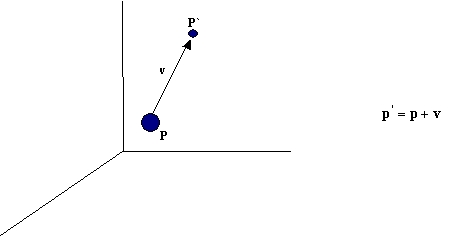
where
p[sup]'[/sup] is the translated point,
p is the original point, and
v is the vector along which to translate.
In matrix form, this turns into:

Where
dx,
dy and
dz are the components of the vector in the respective axis of movement. Note that a 4D vertex is used. These are called
homogeneous co-ordinates, BUT I will not discuss them here.
Scaling
You can scale a vertex by multiplying it by a scalar value, so that
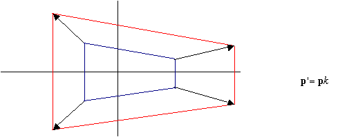
where
k is the scalar constant. You can multiply each component of
p by a different constant. This will make it so you can scale each axis by a different amount.
In matrix form this is:
 Rotation
Rotation is the most complex transformation. Rotation can be performed around the 3 Cartesian axes.
The rotation matrices around these axis are:

To find out more about how these matrices are derived, please pick up a good math book, I haven't got the time to write it here. Some things about these matrices though:
Any rotation about an axis by q can be undone by a successive rotation by -q. So:

Also, notice that the cosine terms are always on the top-left to bottom-right diagonal, and the sine terms are always on the top-right to bottom-left diagonal, we can also say that:

Rotations matrices that act about the origin are orthogonal.
Note that these transformations are cumulative. That is, if you multiplied a vertex by a translation matrix, then by a scale matrix, it would have the effect of moving the vertex, then scaling it. The order that you multiply becomes very important when you multiply rotation and translation matrices together, as
RT does NOT equal
TR!
Projection Matrices
These are also complicated matrices. They come in two flavours,
perspective correct and
orthographic. There are some very good books that derive these matrices in an understandable way, so I won't cover it here. Since I don't work with projection matrices very often, I had to look a lot of this material up using the book
Interactive Computer Graphics by Edward Angel. A very good book that I suggest you buy.
Anyway, on to the matrices.
The orthographic projection matrix:
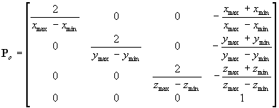
The
x,
y and
z max/min variables define the viewing volume.
The perspective correct projection matrix is:
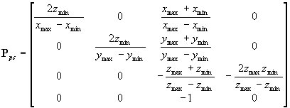
[size="5"]
Conclusion
Well, that's it for this tutorial. I hope that I've helped you understand vectors and matrices including how to use them. For further reading I can recommend a few books that I have found really useful, these are:
Interactive Computer Graphics - A Top Down Approach with OpenGL" - Edward Angel: Covers a lot of theory in computer graphics, including how we perceive the world around us. This book covers a lot of the matrix derivations that I left out. All in all, a very good book on graphics programming and theory. With exercises too, which is nice.
Mathematics for Computer Graphics Applications - Second Edition - M.E Mortenson: This is solely about the mathematics behind computer graphics, and explains a lot of material in a very easy to understand manner. There are loads of exercises to keep you occupied. The book explains things such as vectors, matrices, transformations, topology and continuity, symmetry, polyhedra, half-spaces, constructive solid geometry, points, lines, curves, surfaces, and more! A must for anyone serious in graphics programming. You won't see a line of code or pseudo-code though.
Advanced National Certificate Mathematics Vol.: 2 - Pedoe: I don't know whether you can actually get this book anymore, but if you can get a copy! This book explains mathematical concepts well, and is easy to learn from. This book is about general mathematics though, each volume expands on the other. So vol. 1 introduces concepts, vol. 2 expands on them. A book well worth the money (although I have no idea how much it is, as I got my copy off my dad ).
That's about it! I hope I haven't scared you off graphics programming. Most APIs, including Direct3D and OpenGL, will hide some of this away from you.
If you need to contact me at all, my email address is: [email="phil.dadd@btinternet.com"]phil.dadd@btinternet.com[/email]. I don't want any abuse though - if you don't like this tutorial I accept constructive advice only.
[size="5"]Credits
I'd like to give credit to "Advanced National Certificate Mathematics Vol.: 2" as that's where I got the simultaneous equations from in the part on determinants, so I knew the answers were whole, and that they worked out. I would also like to give credit to Miss. A Miller who proof read this tutorial for me.
 .
A vector equation takes the form a= xi + yj + zk
i, j and k are unit vectors in the 3 standard Cartesian directions. i is a unit vector aligned with the x axis, j is a unit vector aligned with the y axis, and k is a unit vector aligned with the z axis. Unit vectors are discussed later.
The coefficients of the i, j and k parts of the equation are the vector's components. These are how long each vector is in each of the 3 axes. This may be easier to understand with the aid of a diagram.
This diagram shows a vector from the origin to the point ( 3, 2, 5 ) in 3D space. The components of this vector are the i, j and k coefficients ( 2, 3 and 5 ). So, in the above example, the vector equation would be:
a = 2i + 3j + 5k
This can also be related to the deltas of a line going through 2 points.
The second way of writing vectors is as column vectors. These are written in the following form
 where x, y and z are the components of that vector in the respective directions. These are exactly the same as the components of the vector equation. So in column vector form, the above example could be written as:
 There are various advantages to both of the above forms, but I will continue to use the column vector form, as it is easier when it comes to matrices. Position vectors are those that originate from the origin. These can define points in space, relative to the origin.
[size="3"]Vector Math
You can manipulate vectors in various ways, including scalar multiplication, addition, scalar product and vector product. The latter two are extremely useful in 3D applications.
There are a few things you should know before moving to the methods above. The first is finding the modulus (also called the magnitude) of a vector. This is basically its length. This can be easily found using Pythagorean theorem, using the vector components. The modulus of a is written |a|.
 in 3D and
  in 2D, where x, y and z are the components of the vector in the 3 axes of movement. Unit vectors are vectors with a magnitude of 1, so |a| = 1.
Addition
Vector addition is pretty easy. All you do is add the respective components together. So for instance, take the vectors:

 The addition of these vectors would be:
 Get it? This can also be represented very easily in a diagram, but I will only consider this in 2D, because it's easier to draw.


 This works in the same way as moving the second vector so that its beginning is at the first vector's end, and taking the vector from the beginning of the first vector to the end of the second one. So, in a diagram, using the above example, this would be:
 This means that you can add multiple vectors together to get the resultant vector. This is used extensively in mechanics for finding resultant forces.
Subtracting
Subtracting is very similar to adding, and is also quite helpful. All you do is subtract the components in one vector from the components in the other. The geometric representation however is very different.
Let
  and
and  Then
Then  The visual representation of this is:
 Here, a and b are set to be from the same origin. The vector c is the vector from the end of the second vector to the end of the first, which in this case is from the end of b to the end of a. It may be easier to think of this as a vector addition.
Where instead of having:
c = a - b
we have
c = -b + a
which, according to what was said about the addition of vectors would produce:
 You can see that putting a on the end of -b has the same result.
Scalar multiplication
Scalar multiplication is easy to come to grips with. All you do is multiply each component by that scalar.
So, say you had the vector a and a scalar k, you would multiply each component by the scalar, getting this result:

 This has the effect of lengthening or shortening the vector by the amount k. For instance, take k = 2; this would make the vector a twice as long. Multiplying by a negative scalar reverses the direction of the vector. You can use scalar multiplication to find the unit vector of another vector. So, take the following example:
 To find the unit vector of this, we would divide a by |a|. Calling the unit vector "b":

 That is the unit vector b in the direction of a. This just scales each of the components, so that the magnitude is equal to 1.
Scalar multiplication is also used in the vector equation discussed earlier. The constants x, y and z are the scalars that scale the i, j and k vectors, before adding them to find the resultant vector.
The Scalar Product (Dot Product)
The scalar product, also known as the dot product, is very useful in 3D graphics applications. The scalar product is written
  and is read "a dot b".
The definition the scalar product is the following:
 Where q is the angle between the 2 vectors a and b. This produces a scalar result, hence the name scalar product. From this you can see that the scalar product of 2 parallel unit vectors is 1, as |a||b| = 1, and cos(0) also is 1. You should also have seen that the scalar product of two perpendicular vectors is 0, as cos(90) = 0, which makes the rest of the expression 0. The geometric interpretation is:
 The scalar product can also be written in terms of Cartesian components., I will not go into how this is derived, but the final, simplified formula of a.b is:


 We can now put these two equations equal to each other, yielding the equation:
 With this, we can find angles between vectors. This is used extensively in the lighting part of the graphics pipeline, as it can see whether a polygon is facing towards or away from the light source. This is also used in deciding what side of planes points are on, which is also used extensively for culling.
The Vector Product (Cross Product)
The vector product, which is also commonly known as the cross product is also useful. The vector product basically finds a vector perpendicular to two other vectors. Great for finding normal vectors to surfaces.
 For those that are already familiar with determinants, the vector product is basically the expansion of the following determinant:
 For those that aren't, the vector product in expanded form is:
 Read "a cross b".
Since the cross product finds the perpendicular vector, we can say that:
i x j = k
j x k = i
k x i = j
Using scalar multiplication along with the vector product we can find the "normal" vector to a plane. A plane can be defined by two vectors, a and b. The normal vector is a vector that is perpendicular to a plane and is also a unit vector. Using the formulas discussed earlier, we have:

 This first finds the vector perpendicular to the plane made by a and b then scales that vector so it has a magnitude of 1. Note however, that there are 2 possible normals to the plane defined by a and b. You will get different results by swapping a and b in the vector product. That is:
 This is a very important point. If you put the inputs the wrong way round, the graphics API will not produce the desired lighting, as the normal will be facing in the opposite direction.
The Vector Equation of a Straight Line
The vector equation of a straight line is very useful, and is given by a point on the line and a vector parallel to it:
 Where p[sub]0[/sub] is a point on the line and v is the vector. t is called the parameter, and scales v. From this it is easy to see that as t varies, a line is formed in the direction of v. If t only takes positive values, then p[sub]0[/sub] is the starting point of the line. Diagrammatically, this is:
 In expanded form, the equation becomes:


 This is called the parametric form of a straight line.
Using this to find the vector equation of a line through two points is easy:
 If t is confined to values between 0 and 1, then what you have is a line segment between the points p[sub]0[/sub] and p[sub]1[/sub].
Using the vector equation we can define planes, and test for intersections. I won't go into planes much here, as there are many tutorials on them elsewhere, I'll just skim over it.
A plane can be defined as a point on the plane, and two vectors that are parallel to the plane, or:
 where s and t the parameters and u and v are the vectors that are parallel to the plane. Using this, it becomes easy to find the intersection of a line and a plane, because the point of intersection must lie on both the line and the plane, so we simply make the two equations equal to each other.
Take the line:
 and the plane:
 To find the intersection point we simply equate, so that:
 Ed. note: The v on the left in the above equation is not the same vector as the v on the right.
We then solve for w, s and t, and then plug into either the line or plane equation to find the point. When testing for a line segment intersection, w must be between 0 and 1.
There are many benefits for using the normal-distance form of a plane too. It's especially useful for testing what sides of a plane points or other shaped objects are. To do this, you dot the normal vector and the position vector of the point being tested, and add the distance of the plane from the origin.
So, if you have the plane
 and the point ( x, y, z ), the point is in front of the plane if
 and behind if it is < 0. If the result equals zero, the point is on the plane. This is used heavily in culling and BSP trees.
[size="5"]Matrices
[size="3"]What is a Matrix anyway?
A matrix can be considered a 2D array of numbers. They take the form:
 Matrices are very powerful, and form the basis of all modern computer graphics, the advantage of them being that they are so fast. We define a matrix with an upper-case bold type letter. Look at the above example. The dimension of a matrix is its height followed by its width, so the above example has dimension 3x3. Matrices can be of any dimensions, but in terms of computer graphics, they are usually kept to 3x3 or 4x4. There are a few types of special matrices; these are the column matrix, row matrix, square matrix, identity matrix and zero matrix. A column matrix is one that has a width of 1, and a height of greater than 1. A row matrix is a matrix that has a width of greater than 1, and a height of 1. A square matrix is when the dimensions are the same. For instance, the above example is a square matrix, because the width equals the height. The identity matrix is a special type of matrix that has values in the diagonal from top left to bottom right as 1 and the rest as 0. The identity matrix is known by the letter [font="Times New Roman"]I[/font], where
 The identity matrix can be any dimension, as long as it is also a square matrix. The zero matrix is a matrix that has all its elements set to 0.
The elements of a matrix are all the numbers in it. They are numbered by the row/column position so that :
 Vectors can also be used in column or row matrices. I will use column matrices here so that it is easier to understand. A 3D vector a in matrix form will use a matrix A with dimension 3x1 so that:
 which you can see is the same layout as using column vectors.
[size="3"]Matrix arithmetic
I won't go into every matrix manipulation, but instead I'll focus on the ones that are used extensively in computer graphics.
Matrix Multiplication
There are two ways to multiply a matrix: by a scalar, and by another conformable matrix. First, let's deal with the matrix/scalar multiplication.
This is pretty easy, all you do is multiply each element by the scalar. So, let A be the original matrix, B be the matrix after multiplication, and k the constant. We perform:
 where i and j are the positions in the matrix.
this can also be written as:
 Multiplying a matrix by another matrix is more difficult. First, we need to know if the two matrices are conformable. For a matrix to be conformable with another matrix, the number of rows in A needs to equal the number of columns in B. For instance, take matrix A as having dimension 3x3 and matrix B having dimension 3x2. These two matrices are conformable because the number of rows in A is the same as the number of columns in B. This is important as you'll see later. The product of these two matrices is another matrix with dimension 3x2. So, in general terms:
Take three matrices A, B and C where C is the product of A and B. A and B have dimension mxn and pxq respectively. They are conformable if n=p. The matrix C has dimension mxq.
You perform the multiplication by multiplying each row in A by each column in B. So let A have dimension 3x3 and B have dimension 3x2.


 So, with that in mind, let's try an example:


 It's as simple as that! Some things to note:
 A matrix multiplied by the identity matrix is the same, so:
 The transpose of a matrix is it flipped on the diagonal from the top left to the bottom right, so for example:
 The transpose of this matrix would be:
 Simple enough eh? And you thought it was going to be hard!
[size="3"]Determinants
I'm going to talk a little bit about determinants now, as they are useful for solving certain types of equations. I will discuss easy 2x2 determinants first.
Take a 2x2 matrix:
 The determinant of a matrix A is written |A| and is:
 For higher dimension matrices, the determinant gets more complicated. Let's discuss a 3x3 matrix. You pass along the first row, and at each element, you discount the row and column that intersects it, and calculate the determinant of the resultant 2x2 matrix multiplied by that value.
So, for example, take this 3x3 matrix:
 Ok then, Step 1: move to the first value in the top row, a[sub]11[/sub] . Take out the row and column that intersects with that value. Step 2: multiply that determinant by a[sub]11[/sub]. So, using diagrams:
Step1:
 Step2:
 We repeat this all along the top row, with the sign in front of the value of the top row alternating between a "+" and a "-", so the determinant of A would be:
 Now, how do we use these for equation solving? Good question. I will first show you how to solve a pair of equations with 2 unknowns.
Take the two equations:
 We first push the coefficients of the variables into a determinant, producing:
 You can see it's laid out in the same way, which makes it easy. Now, to solve the equation in terms of x, we replace the x coefficients in the determinant with the constants k[sub]1[/sub] and k[sub]2[/sub], dividing the result by the original determinant. So, that would be:
 To solve for y we replace the y coefficients with the constants instead.
Let's try an example to see this working:
 We push the coefficients into a determinant, and solve:
 To find x substitute constants into x co-efficients, and divide by D:
 To find y substitute constants into y co-efficients and divide by D:
 See, it's as simple as that! Just for good measure, I'll do an example using 3 unknowns in 3 equations:

 Solve for x:
 Solve for y:
 Solve for z:
 And there we have it, how to solve a series of simultaneous equations using determinants, something that can be very useful.
Matrix Inversion
Equations can also be solved by inverting a matrix. Take the following equations again:
 We push these into 3 matrices to solve:
 Let's give these names such that:
 We need to solve for B, and since there is no "matrix divide" operation, we need to invert the matrix A and multiply it by D, such that:
 Now we need to know how to actually do the matrix inversion. There are many ways to do this, and the way I am going to show you is by no means the fastest.
To find the inverse of a matrix, we need to first find its co-factor. We use a method similar to what we used when finding the determinant. What you do is this: at every element, eliminate the row and column that intersects it, and make it equal the determinant of the remaining part of the matrix. Let's find the first element in a 3x3 matrix. Let's call it c[sub]11[/sub]. We need to get rid of the row and column that intersects this, so that:
 c[sub]11[/sub] will then take the value of the following determinant:
 The sign in front of c[sub]11[/sub] is decided by the expression:
 Where i and j are the positions of the element in the matrix.
That's easy enough isn't it? Thought so J. Just do the same for every element, and build up the co-factor matrix. Done? Good. Now that the co-factor matrix has been found, the inverse matrix can be calculated using the following equation:
 Taking the previous example and equations, let's find the inverse matrix of A.
First, the co-factor matrix C would be:

 and |A| is:
 So A--[sup]-1[/sup] is:
 To solve the equations, we then do:

 We can then find the values of x,y and z by pulling them out of the last matrix, such that x = -62, y = 39 and z = 3, which is what the other method using determinants found.
A matrix is called orthogonal if its inverse equals its transpose.
[size="3"]Matrices in computer graphics
All graphics APIs use a set of matrices to define transformations in space. A transformation is a change, be it translation, rotation, or whatever. Using column a matrix to define a point in space, a vertex, we can define matrices that alter that point in some way.
Transformation Matrices
Most graphics APIs use 3 different types of primary transformations. These are:
 Translation
To translate a point onto another point, there needs to be a vector of movement, so that
 where p[sup]'[/sup] is the translated point, p is the original point, and v is the vector along which to translate.
In matrix form, this turns into:
 Where dx, dy and dz are the components of the vector in the respective axis of movement. Note that a 4D vertex is used. These are called homogeneous co-ordinates, BUT I will not discuss them here.
Scaling
You can scale a vertex by multiplying it by a scalar value, so that
 where k is the scalar constant. You can multiply each component of p by a different constant. This will make it so you can scale each axis by a different amount.
In matrix form this is:
 Rotation
 is the most complex transformation. Rotation can be performed around the 3 Cartesian axes.
The rotation matrices around these axis are:
Rotation
Rotation is the most complex transformation. Rotation can be performed around the 3 Cartesian axes.
The rotation matrices around these axis are:
 To find out more about how these matrices are derived, please pick up a good math book, I haven't got the time to write it here. Some things about these matrices though:
Any rotation about an axis by q can be undone by a successive rotation by -q. So:
 Also, notice that the cosine terms are always on the top-left to bottom-right diagonal, and the sine terms are always on the top-right to bottom-left diagonal, we can also say that:
 Rotations matrices that act about the origin are orthogonal.
Note that these transformations are cumulative. That is, if you multiplied a vertex by a translation matrix, then by a scale matrix, it would have the effect of moving the vertex, then scaling it. The order that you multiply becomes very important when you multiply rotation and translation matrices together, as RT does NOT equal TR!
Projection Matrices
These are also complicated matrices. They come in two flavours, perspective correct and orthographic. There are some very good books that derive these matrices in an understandable way, so I won't cover it here. Since I don't work with projection matrices very often, I had to look a lot of this material up using the book Interactive Computer Graphics by Edward Angel. A very good book that I suggest you buy.
Anyway, on to the matrices.
The orthographic projection matrix:
 The x, y and z max/min variables define the viewing volume.
The perspective correct projection matrix is:
 [size="5"]Conclusion
Well, that's it for this tutorial. I hope that I've helped you understand vectors and matrices including how to use them. For further reading I can recommend a few books that I have found really useful, these are:
Interactive Computer Graphics - A Top Down Approach with OpenGL" - Edward Angel: Covers a lot of theory in computer graphics, including how we perceive the world around us. This book covers a lot of the matrix derivations that I left out. All in all, a very good book on graphics programming and theory. With exercises too, which is nice.
Mathematics for Computer Graphics Applications - Second Edition - M.E Mortenson: This is solely about the mathematics behind computer graphics, and explains a lot of material in a very easy to understand manner. There are loads of exercises to keep you occupied. The book explains things such as vectors, matrices, transformations, topology and continuity, symmetry, polyhedra, half-spaces, constructive solid geometry, points, lines, curves, surfaces, and more! A must for anyone serious in graphics programming. You won't see a line of code or pseudo-code though.
Advanced National Certificate Mathematics Vol.: 2 - Pedoe: I don't know whether you can actually get this book anymore, but if you can get a copy! This book explains mathematical concepts well, and is easy to learn from. This book is about general mathematics though, each volume expands on the other. So vol. 1 introduces concepts, vol. 2 expands on them. A book well worth the money (although I have no idea how much it is, as I got my copy off my dad ).
That's about it! I hope I haven't scared you off graphics programming. Most APIs, including Direct3D and OpenGL, will hide some of this away from you.
If you need to contact me at all, my email address is: [email="phil.dadd@btinternet.com"]phil.dadd@btinternet.com[/email]. I don't want any abuse though - if you don't like this tutorial I accept constructive advice only.
[size="5"]Credits
I'd like to give credit to "Advanced National Certificate Mathematics Vol.: 2" as that's where I got the simultaneous equations from in the part on determinants, so I knew the answers were whole, and that they worked out. I would also like to give credit to Miss. A Miller who proof read this tutorial for me.
