Preface
This article is designed for those who need to brush up on your maths. Here we will discuss vectors, the operations we can perform on them, and why we find them so useful. We'll then move onto what matrices and determinants are, and how we can use them to help us solve systems of equations. Finally, we'll move onto using matrices to define transformations in space.
This article was originally published to GameDev.net back in 2002. It was revised by the original author in 2008 and published in the book Beginning Game Programming: A GameDev.net Collection, which is one of 4 books collecting both popular GameDev.net articles and new original content in print format.
Vectors
Vector Basics - What is a vector?
Vectors are the backbone of games. They are the foundation of graphics, physics modelling, and a number of other things. Vectors can be of any dimension, but are most commonly seen in two, three, or four dimensions. They essentially represent a direction, and a magnitude. Thus, consider the velocity of a ball in a football game. It will have a direction (where it's travelling), and a magnitude (the speed at which it is travelling). Normal numbers (i.e. single dimensional numbers) are called
scalars.
The notation for a vector is that of a bold lower-case letter, like
i, or an italic letter with an underscore, like
i. I'll use the former in this text. You can write vectors in a number of ways, however I'll only use two here: vector equations and column vectors.
Vectors can be written in terms of its starting and ending position, using the two end points with an arrow above them. So, if you have a vector between the two points A and B, you can write that as:

A vector equation takes the form:
a = x
i + y
j + z
k
The coefficients of the
i,
j, and
k parts of the equation are the vectors
components. These are how long each vector is in each of the 3 axis.
For example, the vector equation pointing to the point ( 3, 2, 5 ) from the origin ( 0, 0, 0 ) in 3D space would be:
a = 2
i + 3
j + 5
k
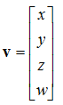
The second way I will represent vectors is as
column vectors. These are vectors written in the following form:

Where
x,
y, and
z are the components of that vector in the respective directions. These are exactly the same as the respective components of the vector equation. Thus in column vector form, the previous example could be written as:

There are various advantages to both of the above forms, although column vectors will continue to be used. Various mathematic texts may use the vector equation form.
Vector Mathematics
There are many ways in which you can operate on vectors, including scalar multiplication, addition, scalar product, vector product and modulus.
Modulus
The
modulus or
magnitude of a vector is simply its length. This can easily be found using Pythagorean Theorem with the vector components. The modulus is written like so:
a = |
a|
Given:
Then,
Where
x,
y and
z are the components of the vector in the respective axis.
Addition
Vector addition is rather simple. You just add the individual components together. For instance, given:

The addition of these vectors would be:
This can be represented very easily in a diagram, for example:


This works in the same way as moving the second vector so that its beginning is at the first vector's end, and taking the vector from the beginning of the first vector to the end of the second one. So, in a diagram, using the above example, this would be:

This means that you can add multiple vectors together to get the resultant vector. This is used extensively in mechanics for finding resultant forces.
Subtracting
Subtracting is very similar to adding, and is also quite helpful. The individual components are simply subtracted from each other. The geometric representation however is quite different from addition. For example:


The visual representation is:
Here,
a and
b are set to be from the same origin. The vector
c is the vector from the end of the second vector to the end of the first, which in this case is from the end of
b to the end of
a.
It may be easier to think of this as a vector addition, where instead of having:
c =
a -
b
We have:
c = -
b +
a
Which according to what was said about the addition of vectors would produce:
You can see that putting
a on the end of -
b has the same result.
Scalar Multiplication
This is another simple operation; all you need to do is multiply each component by that scalar. For example, let us suggest that you have a vector
a and a scalar
k. To perform a scalar multiplication you would multiply each component of the vector by that scalar, thus:

This has the effect of lengthening or shortening the vector by the amount
k. For instance, take
k = 2; this would make the vector a twice as long. Multiplying by a negative scalar reverses the direction of the vector.
The Scalar Product (Dot Product)
The
scalar product, also known as the
dot product, is very useful in 3D graphics applications. The scalar product is written:

This is read "a dot b".
The definition of the scalar product is:
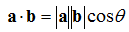
? is the angle between the two vectors
a and
b. This produces a scalar result, hence the name scalar product. This operation has the result of giving the length of the projection of
a on
b. For example:
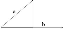
The length of the thick gray horizontal line segment would be the dot product.
The scalar product can also be written in terms of Cartesian components as:


We can put the two dot product equations equal to each other to yield:
With this, we can find angles between vectors.
Scalar products are used extensively in the graphics pipeline to see if triangles are facing towards or away from the viewer, whether they are in the current view (known as frustum culling), and other forms of culling.
The Vector Product (Cross Product)
The
vector product, also commonly known as the
cross product, is one of the more complex operations performed on vectors. In simple terms, the vector product produces a vector that is perpendicular to the vectors having the operation applied. Great for finding normal vectors to surfaces!
I'm not going to get into the derivation of the vector product here, but in expanded form it is:

Read "a cross b".
Since the cross product finds the perpendicular vector, we can say that:
i x
j =
k
j x
k =
i
k x
i =
j
Note that the resultant vectors are perpendicular in accordance with the "right hand screw rule". That is, if you make your thumb, index and middle fingers perpendicular, the cross product of your middle finger with your thumb will produce your index finger.
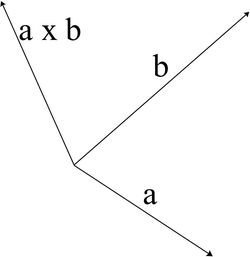
Using scalar multiplication along with the vector product we can find the "normal" vector to a plane. A plane can be defined by two vectors,
a and
b. The normal vector is a vector that is perpendicular to a plane and is also a unit vector. Using the formulas discussed earlier, we have:
c =
a x
b

This first finds the vector perpendicular to the plane made by
a and
b then scales that vector so it has a magnitude of 1.
One important point about the vector product is that:

This is a very important point. If you put the inputs the wrong way round then you will not get the correct normal.
Unit Vectors
These are vectors that have a unit length, i.e. a modulus of one. The
i,
j and
k vectors are examples of unit vectors aligned to the respective axis. You should now be able to recognise that vector equations are quite simply just that. Adding together 3 vectors scaled by varying degrees to produce a single resultant vector.
To find the unit vector of another vector, we use the modulus operator and scalar multiplication like so:

For example:

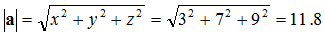
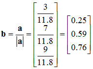
That is the unit vector
b in the direction of
a.
Position Vectors
These are the only type of vectors that have a position to speak of. They take their starting point as the origin of the coordinate system in which they are defined. Thus, they can be used to represent points in that space.
The Vector Equation of a Straight Line
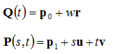
The vector equation of a straight line is very useful, and is given by a point on the line and a vector parallel to it:

Where
p0 is a point on the line, and
v is the unit vector giving its direction.
t is called the parameter and scales
v. From this you can see that as
t varies a line is formed in the direction of
v.
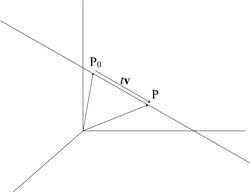
This equation is called the
parametric form of a straight line. Using this to find the vector equation of a line through two points is easy:
If
t is constrained to values between 0 and 1, then we have a
line segment starting at the point
p0 and
p1.
Using the vector equation we can define planes and test for intersections. A plane can be defined as a point on the plane, and two vectors that are parallel to the plane.
Where
s and
t are the parameters, and
u and
v are the vectors that are parallel to the plane. Using this, you can find the intersection of a line and a plane, as the point of intersection must line on both the plane at the line. Thus, we simply make the two equations equal to each other.
Given the line and plane:
To find the intersection we equate so that:
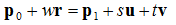
We then solve for
w,
s and
t, and plug them into either the line or plane equation to find the point. When testing for a line segment
w must be in the range 0 to 1.
Another representation of a plane is the normal-distance. This combines the normal of the plane, and its distance from the origin along that normal. This is especially useful for finding out what sides of a plane points are. For example, given the plane
p and point
a:
p =
n +
d
Where,

The point
a is in front of the plane
p if:
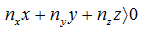
This is used extensively in various culling mechanisms.
Matrices
What is a Matrix anyway?
A matrix can be considered a 2D array of numbers, and take the form:
Matrices are very powerful, and form the basis of all modern computer graphics. We define a matrix with an upper-case bold type letter, as shown above. The dimension of a matrix is its height followed by its width, so the above example has dimension 3x3. Matrices can be of any dimensions, but in terms of computer graphics, they are usually kept to 3x3 or 4x4. There are a few types of special matrices; these are the
column matrix,
row matrix,
square matrix,
identity matrix and
zero matrix. A column matrix is one that has a width of 1, and a height of greater than 1. A row matrix is a matrix that has a width of greater than 1, and a height of 1. A square matrix is when the dimensions are the same. For instance, the above example is a square matrix, because the width equals the height. The identity matrix is a special type of matrix that has values in the diagonal from top left to bottom right as 1 and the rest as 0. The identity matrix is known by the letter
I, where:

The identity matrix can be any dimension, as long as it is also a square matrix.
The
elements of a matrix are all the numbers within it. They are numbered by the row/column position such that:
The zero matrix is one that has all its elements set to 0.
Vectors can also be used in column or row matrices. I will use column matrices here, as that is what I have been using in the previous section. A 3D vector
a in matrix form will use a matrix
A with dimension 3x1 so that:

Which as you can see is the same layout as using column vectors.
Matrix Arithmetic
I'm not going to go into every possible matrix manipulation (we would be here some time), instead I'll focus on the important ones.
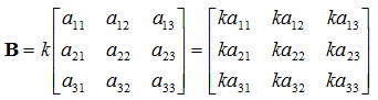
Scalar / Matrix Multiplication
To perform this operation all you need to do is simply multiply each element by the scalar. Thus, given matrix
A and scalar
k:

 Matrix / Matrix Multiplication
Multiplying a matrix by another matrix is more difficult. First, we need to know if the two matrices are
conformable. For a matrix to be conformable with another matrix, the number of rows in
A needs to equal the number of columns in
B. For instance, take matrix
A as having dimension 3x3 and matrix
B having dimension 3x2. These two matrices are conformable because the number of rows in
A is the same as the number of columns in
B. This is important as you'll see later. The product of these two matrices is another matrix with dimension 3x2.
So generally, given three matrices
A,
B and
C, where
C is the product of
A and
B.
A and
B have dimension
mx
n and
px
q respectively. They are conformable if
n=
p. The matrix
C has dimension
mx
q. It is said that the two matrices are conformable if their
inner dimensions are equal (
n and
p here).
The multiplication is performed by multiplying each row in
A by each column in
B. Given:
So, with that in mind let us try an example!

It's as simple as that! Some things to note:

A matrix multiplied by the identity matrix is the same, so:
AI =
IA =
A
The Transpose
The
transpose of a matrix is it flipped along the diagonal from the top left to the bottom right and is denoted by using a superscript
T, for example:

Determinants
Determinants are a useful tool for solving certain types of equations, and are used rather extensively.
Let's take a 2x2 matrix
A:
The determinant of matrix
A is written |
A| and is defined to be:
That is the top left to bottom right diagonal multiplied together subtracting the top right to bottom left diagonal. Things get a bit more complicated with higher dimensional determinants, let us discuss a 3x3 determinant first. Take
A as:

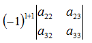
Step 1: move to the first value in the top row, a11. Take out the row and column that intersects with that value.

Step 2: multiply that determinant by a11.

We repeat this along the top row, with the sign in front of the result of step 2 alternating between a "+" and a "-". Given this, the determinant of
A becomes:

Now, how do we use these for equation solving? Good question.
Given a pair of simultaneous equations with two unknowns:

We first
push these coefficients of the variables into a determinant, producing:

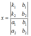
You can see that it is laid out in the same way. To solve the equation in terms of
x, we replace the
x coefficients in the determinant with the constants
k1 and
k2, dividing the result by the original determinant:
To solve for
y we replace the
y coefficients with the constants instead. This algorithm is called
Cramers Rule.
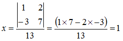
Let's try an example to see this working, given the equations:
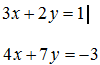
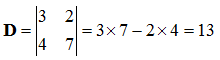
We push the coefficients into a determinant and solve:
To find
x substitute the constants into the
x coefficients, and divide by
D:
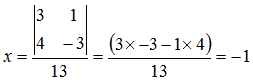
To find
y substitute the constants into the
y coefficients, and divide by
D:
It's as simple as that! For good measure, let's do an example using 3 unknowns in 3 equations:
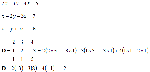
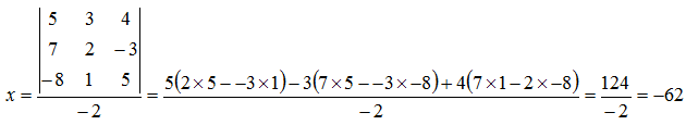
Solve for
x:
Solve for
y:
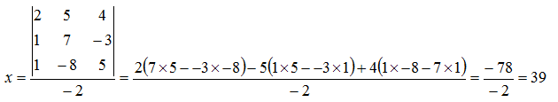
Solve for
z:
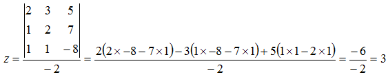
And there we have it, how to solve a series of simultaneous equations using determinants, something that can be very useful.
Matrix Inversion
Equations can also be solved by inverting a matrix. Using the same equations as before:
We first push these into three matrices to solve:
Let's give these names such that:

We need to solve for
B (this contains the unknowns after all). Since there is no "matrix divide" operation, we need to invert
A and multiply it by
D such that:

Now we need to know how to actually do the matrix inversion. There are many ways to do this, and the way that I'm going to use here is by no means the fastest.
To find the inverse of a matrix, we need to first find its
co-factor. We use a method similar to what we used when finding the determinant. What you do is this: at every element, eliminate the row and column that intersects it, and make it equal the determinant of the remaining part of the matrix, multiplied by the following expression:

Where
i and
j is the position in the matrix.
For example, given a 3x3 matrix
A, and its co-factor
C. To calculate the fist element in the cofactor matrix (c11), we first need to get rid of the row and column that intersects this so that:
c11 would then take the value of the following:
We would then repeat for all elements in matrix
A to build up the co-factor matrix
C. The inverse of matrix
A can then be calculated using the following formula.

The transpose of the co-factor matrix is also referred to as the
adjoint.
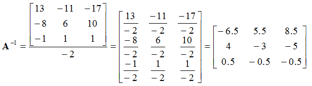
Given the previous example and equations, let's find the inverse matrix of
A.
Firstly, the co-factor matrix
C would be:

|
A| is:
|
A| = -2
Thus, the inverse of
A is:
We can then solve the equations by using:


We can find the values of
x,
y and
z by pulling them out of the resultant matrix, such that:
x = -62
y = 39
z = 3
Which is exactly what we got by using Cramer's rule!
Matrices are said to be
orthogonal if its transpose equals its inverse, which can be a useful property to quick inverting of matrices.
Matrix Transformations
Graphics APIs use a set of matrices to define transformations in space. A transformation is a change, be it translation, rotation, or whatever. Using position vector in a column a matrix to define a point in space, a
vertex, we can define matrices that alter that point in some way.
Transformation Matrices
Most graphics APIs use three different types of primary transformations. These are translation; scaling; and rotation. We can transform a point
p using a transformation matrix
T to a point
p' like so:
p' =
Tp
We use 4 dimensional vectors from now on, of the form:
We then use 4x4 transformation matrices. The reason for the 4th component here is to help us perform translations using matrix multiplication. These are called
homogeneous coordinates. I won't go into their full derivation here, as that is quite beyond the scope of this article (their true meaning and purpose comes from points in projective space).
Translation
To translate a point onto another point, there needs to be a vector of movement, so that:
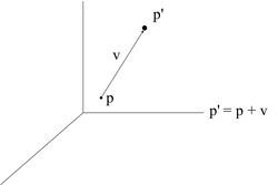
Where
p' is the translated point,
p is the original point and
v is the vector along which the translation has taken place.
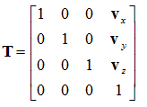
By keeping the w component of the vector as 1, we can represent this transformation in matrix form as:
 Scaling
You can scale a vertex by multiplying it by a scalar value, such that:
Where
k is the scalar constant. You can multiply each component of
p by a different constant. This will make it so you can scale each axis by a different amount.
In matrix form this becomes:
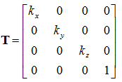
Where
kx,
ky, and
kz are the scaling factors in the respective axis.
Rotation
Rotation is a more complex transformation, so I'll give a more thorough derivation for this than I have the others.
Rotation in a plane (i.e. in 2D) can be described in the following diagram:
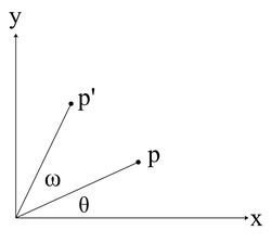
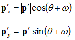
This diagram shows that we want to rotate some point
p by ? degrees to point
p'. From this we can deduce the following equations:
We are dealing with rotations about the origin, thus the following can be said:
|
P'| = |
P|
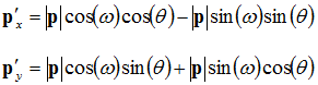
Using the trigonometric identities for the sum of angles:
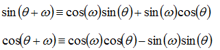
We can expand the previous equations to:
From looking at the diagram, you can also see that:
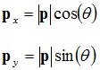
Substituting those into our equations, we end up with:
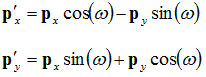
Which is what we want (the second point as a function of the first point).
We can then push this into matrix form:
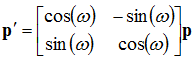
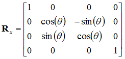
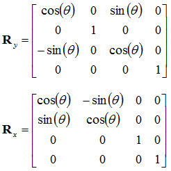
Here, we have the rotation matrix for rotating a point in the x-y plane. We can expand this into 3D by having three different rotation matrices, one for rotating along the x axis, one in the y axis, and another for the z axis (this one is effectively what we have just done). The unused axis in each rotation remains unchanged. These rotation matrices become:
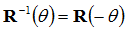
Any rotation about an axis by ? can be undone by a successive rotation by -?, thus:
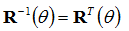
Also, notice that the cosine terms are always on the top left to bottom right diagonal, and notice the symmetry of the sine terms along this axis. This means, we can also say:
Rotation matrices that act upon the origin are orthogonal.
One important point to consider is the order of rotations (and transformations in general). A rotation along the x axis followed by a rotation along the y axis is
not the same as if it were applied in reverse. Similarly, a translation followed by a rotation does
not produce the same result as a rotation followed by a translation.
Frames
A frame can be considered a local coordinate system, or
frame of reference. That is, a set of three
basis vectors (unit vectors perpendicular to each other), plus a position, relative to some other frame. So, given the basis vectors and position:
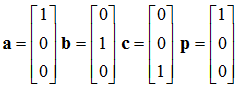
That is
a,
b, and
c defines the basis vectors, with
p being its position.
We can push this into a matrix, defining the frame, like so:
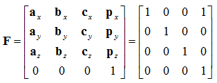
This matrix is useful, as it lets us transform points into a second frame - so long as those points exist in the same frame as the second frame. Thus, consider a point in some frame:
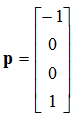
Assuming the frame we defined above is in the same frame as that point, we can transform this point to be in our frame like so:

That is:
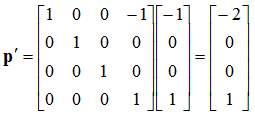
Which if you think about it is what you would expect. If you have a point at -1 along the x axis, and you transform it into a frame that is at +1 along the x axis and orientated the same, then
relative to that second frame the point appears at -2 along
its x axis.
This is useful for transforming vertices between different frames, and is incredibly useful for having objects moving relative to one frame, while that frame itself is moving relative to another one. You can simply multiply a vertex first by its parent frame, then by its parents frame, and so forth to eventually get its position in
world space, or the global frame.
You can also use the standard transformation matrices previously to transform frames with ease. For instance, we can transform the above frame to rotate by 90? along the y axis like so:
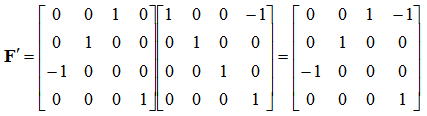
This is exactly what you would expect (the z axis to move to where the x axis was, and the x axis point in the opposite direction to the original z axis).
Summary
Well that's it for this article. We've gone through what vectors are, the operations that we can perform on them and why we find them useful. We then moved onto matrices, how they help us solve sets of equations, including how to use determinants. We then moved on to how to use matrices to help us perform transformations in space, and how we can represent that space as a matrix.
I hope you've found this article useful!
References
Interactive Computer Graphics - A Top Down Approach with OpenGL - Edward Angel
Mathematics for Computer Graphics Applications - Second Edition - M.E Mortenson
Advanced National Certificate Mathematics Vol.: 2 - Pedoe


I'm going through Differential Geometry by Graustein right now. Another easy to understand method of the determinant for a 3x3 is the outer product between the first 2 basis vectors, follow by an inner product between the resultant vector and the 3rd basis. Seeing that finally made me understand what the determinant actually is.
I would love to see another article giving the derivation of the homogenous 4d coordinate systems, as projective geometry is still a weak area for me.