Coefficients for bezier curves

Started by
6 comments, last by cadjunkie 10 years, 11 months ago
I have been working with Cubic and Quadratic bezier curves for the past week, and one thing that I am still not sure about is how to get the polynomial coefficients from the control points. For example, a cubic bezier has the formula A*t^3 + B*t^2 + C*t + D and a quadratic one has A*t^2 + B*t + C. The cubic bezier is defined by the end points P0 and P3, and the control points P1 and P2. The quadratic one is just P0, P1 and P2. http://floris.briolas.nl/floris/2009/10/bounding-box-of-cubic-bezier/ says that the coefficients for the cubic bezier can be calculated like:
m_DX = m_P0.x;
m_CX = 3.0f * ( m_P1.x - m_P0.x );
m_BX = ( 3.0f * m_P2.x ) - ( 6.0f * m_P1.x ) + ( 3.0f * m_P0.x );
m_AX = m_P3.x - ( 3.0f * m_P2.x ) + ( 3.0f * m_P1.x ) - m_P0.x;
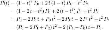
These coefficients can be plugged into the formula A*t^3 + B*t^2 + C*t + D and it works, so they seem to be okay. I am not sure how those coefficients were derived though. Can anyone explain this to me? Also, I would need to calculate the same coefficients for a quadratic bezier.
Thanks!
Advertisement

You start from the parametric Bézier curve formula and rewrite the terms until you obtain the desired formula. This is simple algebra, nothing complicated. For example, for the quadratic case:

acv2qqk.png

The derivation in the cubic case is similar. But I have always found the Bézier formula a much more useful formulation. Why do you want the coefficients of the polynomial?

EDIT: corrected the formula..

Thanks, I'll have to look through that. I am using the coefficients for several things. For example, to get the x at a given t I can just do:


float Curve::QuadraticBezierSegment::getXAtT( float t ) const
{
// A*t^2 + B*t + C
return ( m_AX * t * t ) + ( m_BX * t ) + m_CX; 
}
 

There might be some other way to do that too, I am not sure. Also, if I take the derivative of the formula and plug in the coefficients I can solve it and get local extrema, ie. the bounds of the curve. Again, I am not a math person, and there might be other ways to do this. If some come to mind, please feel free to share smile.png

To get a point in a Bézier curve the standard method is known as De Casteljau's algorithm. You iteratively linearly interpolate all control points until you find a single point. This is more robust than evaluating your formula. It is also useful to get a better geometric intuition. You may also be interested in the Horner's Method which is a more robust way to evaluate your polynomial. You write C + t*(B + t*A) instead of C + t*B + t*t*A in the quadratic case.

The derivative of a Bézier curve is a lower degree Bézier curve. The derivative of a quadratic Bézier curve is thus a segment and of a cubic Bézier curve is a quadratic Bézier curve. The proof use the following result on the Bernstein polynomials (used to define the equation of a Bézier curve).

clnba7b.png

The control points of the derivative curve are indeed the points a9lcbze.png for all i from 0 to n-1.

If all you want is however to get some bounds on the curve, a Bézier curve also have the property to be contained in the convex hull of its points. It can be useful to easily discard curve pairs for collision for example. There also exists interative methods to compute intersections of Bézier curve using this method (or something similar).

Coolio, thanks for the explanation!

(Disclaimer: sorry if the LaTeX equations don't come out right; I've had issues!)

apatriarca's formula for the derivative of a Bezier curve is mostly right, but you need to divide the control points by the interval of the curve. The formula for the derivative's control points is Di = n/(t1 - t0) * (Pi+1-Pi). This isn't a problem if the parameter domain for the Bezier curve is [0,1], but if it's something else, then you have to divide by the interval.

If you want to convert a Bezier curve to a power basis polynomial, you need to convert the Bezier curve into an explicit Bezier curve (one where the x-coordinates of the curve are evenly spaced, such as below:

[attachment=15778:explicit.jpg]

Then you can express this as a Bernstein polynomial [eqn]y = \sum_{i=0}^n y_i B_i^n (t)[\eqn], where x = t. The closed-form conversion between Bernstein to power basis is given as [eqn]p_i = \sum_{k=0}^i b_k \binom{n}{i} \binom{i}{k} (-1)^{i-k}[\eqn].

My real question is: why you would want to convert to a polynomial when you can probably do what you want in the Bernstein basis?

In my previous reply I was only considering Bézier curves in which t vary uniformly in the [0, 1] interval. If you change the parametrization you clearly have to adjust the derivative, but this does not make my result wrong in any way. More complicated parametrizations are actually also possible. What if I want to use t = sin(s) with s in [0, pi/2]? The (support of the) curve clearly remains the same, but the velocity/derivative is now different.

apatriarca, I didn't mean to say that your formula was incorrect. I just wanted to add that the interval of the curve matters in the derivative, you know, for completeness.

This topic is closed to new replies.

Advertisement