In 2005 I spent a good amount of time answering questions in the "For Beginners" forums of GameDev.net.
One question which I frequently saw was how to compute the vertex normals required for various diffuse lighting models used in games. After answering the question three or four times, I aimed to write an introductory article which would explain the most commonly used algorithms for computing surface and vertex normals to date and to compare and contrast their performance and rendering quality. However, times and technology have changed.
At the time of my first article, Real-Time Shaders were just becoming the de-facto standard method for implementing graphics amongst video game developers, and the lack of texture fetches for Vertex Shaders and the limited instruction count prevented people from performing many of the operations they would have liked on a per-frame basis directly on the GPU.
However, with the introduction of DirectX 10, Geometry Shaders, Streamed Output, and Shader Model 4.0 it's now possible to move the work-load of transforming and lighting our scenes entirely to the GPU.
In this article, we will be utilizing the new uniform interface for texture fetching and shader resources of DirectX 10, along with the new Geometry Shader Stage to allow us to efficiently compute per-frame, per vertex normals for dynamic terrain such as rolling ocean waves or evolving meshes - entirely on the GPU. To make sure we cover our bases will we be computing the normals for terrain lighting using two distinct algorithms, each of which addresses a specific type of terrain.
It is my hope that by the end of this article you will have discovered some efficient and exciting ways to take advantage of current-generation hardware to compute the surface and vertex normals necessary for the complex lighting algorithms which will be popping up with the new generation of rendering hardware.
This article was originally published to GameDev.net in 2005. It was revised by the original author in 2008 and published in the book Advanced Game Programming: A GameDev.net Collection, which is one of 4 books collecting both popular GameDev.net articles and new original content in print format.
Heightmap Based Terrain
Depending upon the genre of game you're making, players may spend a significant amount of time looking at the terrain or ocean waves passing them by. With this in mind, it is desirable to have a terrain which is both realistic and attractive to look at. Among the simplest methods of creating attractive terrain are those based on heightmaps.
A heightmap is a one or two dimensional array of data which represents the height of a piece of terrain at a specific (x, z) point in space. In other words, if you were to look at the [x][z] offset within a 2D array or compute the associated index into a one-dimensional array, the value at that location in memory would be the height at point X, Z in 3D space.
The value in memory can be stored as either a floating point value or an integer, and in the case of an integer the values are often stored as either a 1 byte (8 bits) or 4 byte (32 bits) block of memory. When the height values are stored as 8-bit integers the heightmap can easily be saved and loaded to disk in the form of a grayscale image. This makes it possible to use a standard image editing application to modify the terrain offline. Figure 1 shows an example grayscale Heightmap.
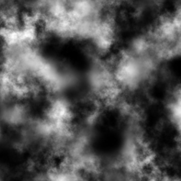 Figure 1: An example heightmap taken from Wikipedia
Fortunately for us, technology has advanced a great deal in recent years, and floating point buffers and textures are now frequently used. For the purpose of this article, we will use 32 bit, single precision Floating Point values to represent height. When working with static terrain, or when it's necessary to perform collision detection, the values from the heightmap can be read from memory and then assigned to a grid-shaped mesh that contains the same number of rows and columns of vertices as the dimension of the heightmap.
Once this is done, the newly generated mesh can be triangulated and passed to the renderer for drawing or can be used for picking and collision detection. This "field of vertices" which is used for rendering and collision is called the heightfield. You can see a 3D heightfield representation of the heightmap used above in Figure 2.
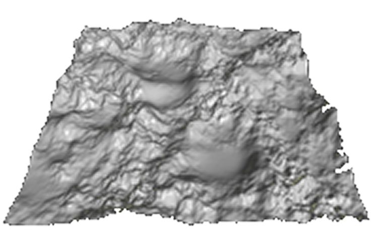 Figure 2: An example 3D heightfield taken from Wikipedia
Because the distance between pixels in a heightmap are unfirormly treated as one, it is common to generate a heightfield with similarly distributed vertices. However, forcing your vertices to exist in increments of one can cause the terrain to seem unnatural.
For this reason, a horizontal scale factor, sometimes called "Scale" or "Units per Vertex" is added to allow your vertices to be spaced in distances greater or smaller than 1.0. When it is not necessary for actors to collide against the terrain, or when it's possible for the collisions to be computed on the GPU, it is more common to pass the heightmap directly to the GPU along with a flat mesh.
In this case, the scaling and displacement of the vertices is performed by the GPU and is referred to as Displacement Mapping. This is the method we'll use in this article.
Slope Method of Computing Heightfield Normals
Because heightfields are generated from heightmaps, the vertices are always evenly spaced and are never overlapping (resulting in the y-component of our normal always facing "up"). This makes it possible to break our 3-dimensional heightfield into two, 2-dimensional coordinate systems, one in the XY plane, and one in the ZY plane.
We can then use the simple and well-known phrase "rise above run" from elementary geometry to compute the x and z component normals from each of our coordinate systems, while leaving the y-component one. Consider the line shown in figure 3.
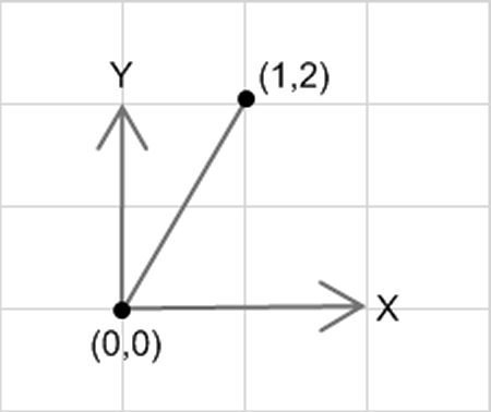 Figure 3: A simple 2D line
In figure 3 you can see that the slope for the line segment is 2. If you assume for a moment that the line segment represents a 3D triangle laying on its side, and that the front face of the triangle points "up", then the surface normal for such a triangle (in the x-direction) can be determined by finding the negative reciprocal of the slope.
In this case, the negative reciprocal is -(1/2). At the beginning of this explanation I made a point of indicating that we can express our 3D heightfield as a pair of 2D coordinate systems because the Y component of our normal always points up. That implies that we want to keep our y-component positive. So the slope for our normal is better expressed as 1 / -2.
Note that this means our dy is 1 and dx is -2, and that if we use those values as the x and y components of a 2D normal vector we get the vector (-2, 1).
Once normalized, that would indeed represent a vector which is normal to the triangle lying on its side in the XY plane. In the discussion of heightfields we also noted that the distance between pixels is always 1, and consequently, the distance between vertices in the heightfield (before scaling) is also one. This further simplifies our computation of normals because it means that the denominator of our expression "rise / run" is always one, and that our x-component can be computed simply by subtracting the y-components (the rise) of the two points which make up our line segment.
Assume y is 1, and then subtract our first height (1) from our first height (3), and you get -2. So now we have a fast and efficient method of computing the normal for a line segment, the 2D equivalent of a surface normal, but we still need to take one more step to compute the normal for each vertex. Consider the picture in Figure 4.
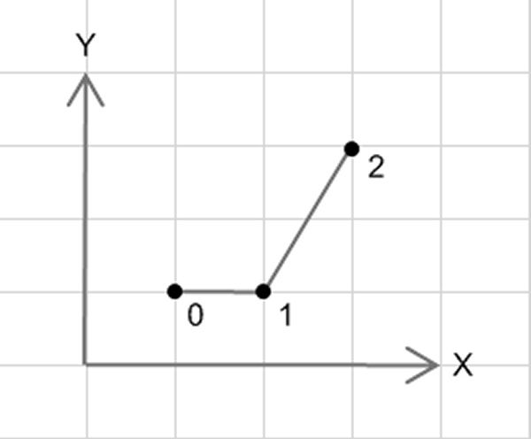 Figure 4: A series of 2D line segments
Here you can see 3 vertices, each separated by a line segment. Visually, the normal at point 0 would just be the up vector, the normal at point 2 would be the same as the line segment which we computed previously, and point 1 would be half-way in between. From this observation we can generalize an algorithm for computing the component-normal for a point in a 2D coordinate system.
"The vertex normal in a 2D coordinate system is the average of the normals of the attached line segments."
Or, when expressed using standard equation speak:
ComponentNormal = ? (lineNormals) / N; where N is the number of normals
Up until this point I've attempted to consistently use the term "component normal" to remind you that what we've been computing so far is simply the X-component of the normal in our 3D heightfield at any given vertex. Fortunately for us, computing the Z component is exactly the same.
That is, we can compute the dy in the z-direction to get the z-component of the normal, just like we computed dy in the x-direction to get the x-component. When we combine the two equations, we get the following:
Normal.x = ?(x-segments) / Nx; Normal.y = 1.0 Normal.z = ?(z-segments) / Nz;
The above algorithm can be shown more effectively using a visual aid.
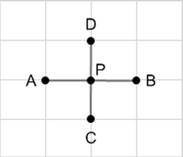 Figure 5: An overhead view of a heightfield
If you take the example shown in Figure 5 you'll see the algorithm can be filled in to get the following equations:
Normal.x = [(A-P) + (P-B)] / 2.0 Normal.y = 1.0 Normal.z = [(C-P) + (P-D)] / 2.0
During implementation, the algorithm becomes a little more complicated because you must:
- Find the indices of your points in the height data
- Handle edge cases in which there are fewer points to sample
Rather than describe the special cases here, let's look at them in the context of an implementation in DirectX 10 using Vertex Shaders.
Implementing the Algorithm with DirectX 10
In the explanation that follows I will try and address the most relevant components of implementing the above algorithm within a DirectX 10 application. However, I will be using the source code from the associated demo program which you may examine for a more complete listing and an idea of how it may fit in into your own games.
Before we do anything else we need to define our custom vertex format. For our 3D heightfield we're only going to need two floating point values, x and z. This is because the normal values, along with the y-component of our position, will be pulled from the heightmap and procedurally computed within our Vertex Shader.
When initializing the x and z components within our program, we are going to set them to simple integer increments, 0, 1, 2... We do this so we can compute an index into our heightmap in order to determine the height at any given vertex.
struct FilterVertex // 8 Bytes per Vertex
{
  float x, z;
};
The index into a one dimensional heightmap can be computed with the following equation, where numVertsWide is how many pixels in your heightmap in the x dimension:
index = z * numVertsWide + x DirectX 10 is unique from DirectX 9 and is particularly suited for this type of problem because unlike DirectX 9 it provides a uniform interfaces for each stage in the graphics pipeline. This allows you create buffers, textures, and constants which can be accessed the same across all stages.
For our particular purpose we're going to need a buffer to store our heights in. In DirectX 9, with Shader Model 3, we could have done this by stuffing our heights into a texture and then accessing it using the SM 3.0 vertex texture fetching operations. However, with DirectX 10 it's even easier. We can define a buffer which will store our heights and then bind it to the graphics pipeline as a Shader Resource. Once we do this, we access the buffer as though it were any other global variable within our shaders. To make this possible we need to define three different fields:
ID3D10Buffer* m_pHeightBuffer;
ID3D10ShaderResourceView* m_pHeightBufferRV;
ID3D10EffectShaderResourceVariable* m_pHeightsRV;
First, we'll need the buffer itself. This is what ultimately contains our float values and what we'll be updating each frame to contain our new heights. Next, all resources which derive from ID3D10Resource (which includes textures and buffers) require an associated Resource View which tells the shader how to fetch data from the resource. While we fill our buffer with data, it is the Resource View which will be passed to our HLSL Effect.
Finally, we're going to need an Effect Variable. In DirectX 10, all effect fields can be bound to one of several variable types. Shader Resources such as generic buffers and textures use the Shader Resource Variable type. While we won't demonstrate it here, you will need to define your vertex and index buffers, and fill them with the corresponding values. Once you've done that you'll want to create the shader resources we previously discussed.
To do this you create an instance of the D3D10_BUFFER_DESC and D3D10_SHADER_RESOURCE_VIEW_DESC structures and fill them in using the following code:
void Heightfield::CreateShaderResources(int numSurfaces)
{
  // Create the non-streamed Shader Resources
  D3D10_BUFFER_DESC desc;
  D3D10_SHADER_RESOURCE_VIEW_DESC SRVDesc;

  // Create the height buffer for the filter method
  ZeroMemory(&desc, sizeof(D3D10_BUFFER_DESC));
  ZeroMemory(&SRVDesc, sizeof(SRVDesc));
  desc.ByteWidth = m_NumVertsDeep * m_NumVertsWide * sizeof(float);
  desc.Usage = D3D10_USAGE_DYNAMIC;
  desc.BindFlags = D3D10_BIND_SHADER_RESOURCE;
  desc.CPUAccessFlags = D3D10_CPU_ACCESS_WRITE;
  SRVDesc.Format = DXGI_FORMAT_R32_FLOAT;
  SRVDesc.ViewDimension = D3D10_SRV_DIMENSION_BUFFER;
  SRVDesc.Buffer.ElementWidth = m_NumVertsDeep * m_NumVertsWide;
  m_pDevice->CreateBuffer(&desc, NULL, &m_pHeightBuffer);
  m_pDevice->CreateShaderResourceView(m_pHeightBuffer, &SRVDesc, &m_pHeightBufferRV);
}
For our filter normal algorithm, we're going to be writing to the heightmap buffer once every frame, so we'll want to specify it as a writeable, dynamic resource. We also want to make sure it's bound as a shader resource and has a format which supports our 32 bit floating point values. Finally, as seen in the code listing, we need to specify the number of elements in our buffer. Unfortunately, the field we use to do this is horribly misnamed and in the documentation is described as containing a value which it should not. The field we're looking for is ElementWidth.
The documentation says it should contain the size of an element in bytes, however this incorrect. This field should contain the total number of elements. Don't be fooled. After we've created our index, vertex, and height buffers and filled them in with the correct values, we'll need to draw our heightfield. But, before we pass our buffers off to the GPU we need to make sure to set the relevant properties for the different stages and set our buffers. So let's examine our draw call a little bit at a time. First, we'll define a few local variables to make the rest of the method cleaner.
void Heightfield::Draw()
{
  // Init some locals
  int numRows = m_NumVertsDeep - 1;
  int numIndices = 2 * m_NumVertsWide;
  UINT offset = 0;
  UINT stride = sizeof(FilterVertex);
Next, we need to tell the vertex shader the dimensions of our heightfield, so that it can determine whether a vertex lies on an edge, a corner, or in the middle of the heightfield. This is important as the number of line segments included in our algorithm is dependent upon where the current vertex lies in the heightfield.
m_pNumVertsDeep->SetInt(m_NumVertsDeep);
m_pNumVertsWide->SetInt(m_NumVertsWide);
m_pMetersPerVertex->SetFloat(m_MetersPerVertex);
Next, we're going to follow the usual procedure of specifying the topology, index buffer, input layout, and vertex buffer for our terrain
m_pDevice->IASetPrimitiveTopology (D3D10_PRIMITIVE_TOPOLOGY_TRIANGLESTRIP);
m_pDevice->IASetIndexBuffer(m_pIndexBuffer,DXGI_FORMAT_R32_UINT,0);
m_pDevice->IASetInputLayout(m_pHeightfieldIL);
m_pDevice->IASetVertexBuffers(0, 1, &m_pHeightfieldVB, &stride, &offset);
Next, and this is perhaps the most important step, we're going to bind the resource view of our buffer to the effect variable established effect variable. Once we've done this, any references to the buffer inside of the HLSL will be accessing the data we've provided within our heightmap buffer.
m_pHeightsRV->SetResource(m_pHeightBufferRV); Finally, we're going get apply the first pass of our technique in order to set the required stages, vertex and pixel shaders, and then we're going to draw our terrain.
m_pFilterSimpleTech->GetPassByIndex(0)->Apply(0);
for (int j = 0; j < numIndices; j++)
{
  DrawIndexed( numIndices, j * numIndices, 0 );
}
In my demo I treated the terrain as a series of rows, where each row contains a triangle strip. Previous to DirectX 10 it might have been better to render then entire heightfield as a triangle list in order to reduce the number of draw calls. However, in DirectX 10 the performance penalty for calling draw has been amortized and is significantly less.
As a result, I chose to use Triangle Strips to reduce the number of vertices being sent to the GPU. Feel free to implement the underlying topology of your heightfield however you like. Now that we've taken care of the C++ code let's move on to the HLSL. The first thing we're going to do is define a helper function which we will use to obtain the height values from our buffer.
The Load function on the templated Buffer class can be used to access the values in any buffer. It takes an int2 as the parameter where the first integer is the index into the buffer, and the second is the sample level. This should just be 0, as it's unlikely your buffer has samples. As I mentioned previously, DirectX 10 provides a uniform interface for many types of related resources. The second parameter of the Load method is more predominately used for Texture objects which may actually have samples.
float Height(int index) { return g_Heights.Load(int2(index, 0)); }
Now that we've got our helper function in place lets implement our filter method. In this method we declare a normal with the y-component facing up, and then we set the x and z values to be the average of the computed segment normals, depending on whether the current vertex is on the bottom, middle, or top rows, and whether it's on the left, center, or right hand side of the terrain. Finally, we normalize the vector and return it to the calling method.
float3 FilterNormal( float2 pos, int index )
{
  float3 normal = float3(0, 1, 0);

  if(pos.y == 0)
    normal.z = Height(index) - Height(index + g_NumVertsWide);
  else if(pos.y == g_NumVertsDeep - 1)
    normal.z = Height(index - g_NumVertsWide) - Height(index);
  else
    normal.z = ((Height(index) - Height(index + g_NumVertsWide)) + (Height(index - g_NumVertsWide) - Height(index))) * 0.5;

  if(pos.x == 0)
    normal.x = Height(index) - Height(index + 1);
  else if(pos.x == g_NumVertsWide - 1)
    normal.x = Height(index - 1) - Height(index);
  else normal.x = ((Height(index) - Height(index + 1)) + (Height(index - 1) - Height(index))) * 0.5;

  return normalize(normal);
}
For each vertex we're going to execute the following vertex shader:
VS_OUTPUT FilterHeightfieldVS( float2 vPos : POSITION )
{
  VS_OUTPUT Output = (VS_OUTPUT)0;
  float4 position = 1.0f;
  position.xz = vPos * g_MetersPerVertex;
First, we take the 2D position which was passed in and compute the index into our buffer. Once we've got the index, we use the Load method on the texture object in order to obtain the height at the current position, and use that to set the y-component of our vertex's position.
// Pull the height from the buffer
int index = (vPos.y * g_NumVertsWide) + vPos.x;
position.y = g_Heights.Load(int2(index, 0)) * g_MetersPerVertex;
Output.Position = mul(position, g_ViewProjectionMatrix);
Next, we pass the 2D position and the index into the previously shown filter method. We pass the index into the function in order to prevent having to compute it again, and we pass in the position as the x and z values are used to determine whether the vertex lies on the edge of the terrain.
  // Compute the normal using a filter kernel
  float3 vNormalWorldSpace = FilterNormal(vPos, index);

  // Compute simple directional lighting equation
  float3 vTotalLightDiffuse = g_LightDiffuse * max(0,dot(vNormalWorldSpace, g_LightDir));
  Output.Diffuse.rgb = g_MaterialDiffuseColor * vTotalLightDiffuse;
  Output.Diffuse.a = 1.0f;
  return Output;
}
As an additional note about this implementation, with DirectX 10 and the introduction of the Geometry Shader it's now possible to generate geometry directly on the GPU. If someone were interested they could completely avoid the need to pass a mesh to the GPU and instead generate it, along with the normals inside of the geometry shader. However, as most games are not bus-bound, there would be no noticeable performance benefit as simply creating a static vertex buffer and passing it to the GPU each frame requires little overhead by the CPU.
Mesh-Based Terrain
While the previous algorithm works effectively for heightmap based terrain, it's unacceptable for mesh-based terrain. In this case, caves, chasms, overhangs, and waves prevent us from performing any type of optimizations because we can make no guarantees about the direction of the y-component. For this reason it becomes necessary to compute the full normal. The following algorithm is a fast and efficient method for computing cross-products for mesh-based terrain entirely on the GPU, so long as certain assumptions and constraints are made.
Grid-Mesh Smooth Shading Algorithm
I refer to this algorithm as the Grid-Mesh Smooth shading algorithm because it is a combination of two principles. The first principle, which results in the "Smooth Shading" part of the name, was set forth by Henri Gouraud. Gouraud suggested that if you were to compute the normals of each of the facets (surfaces) of a polyhedron then you could get relatively smooth shading by taking all of the facets which are "attached" to a single vertex and averaging the surface normals.
Gouraud Shading is thus a two stage algorithm for computing the normal at a vertex. The first stage is to compute the surface normals of each of the triangles in the heightfield using cross-product calculations. The second stage is to sum the surface normals attached to any given vertex and then normalize the result. The following two equations are the mathematical definitions for the surface and vertex normals.
Surface Normal: Ns - A x B Vertex Normal: N = Norm( - (Nsi) )
While I won't demonstrate all the methods here (though they are included in the associated demo), there are actually three different ways for computing the vertex normals which distribute the workload differently. In order of efficiency they are:
- Compute both the surface and vertex normals on the CPU
- Compute the surface normals on the CPU and the vertex normals on the GPU
- Compute both the surface and vertex normals on the GPU
Until DirectX 10, only the first two options were available, and were still expensive as computing the cross-products for a large number of triangles on the CPU each frame can become unreasonable.
With DirectX 10 and Geometry Shaders it is now possible to compute both the surface and vertex normals entirely on the GPU. This method is significantly faster than computing the surface normals on the CPU and allows us to get much closer in performance of complex, mesh-based terrain to the methods used for heightmap based terrain.
The Geometry Shader Stage is unique in its functionality in that, unlike the Vertex Shader Stage which receives a single vertex at a time, or the Pixel Shader Stage which receives a single pixel at a time, the Geometry Shader Stage can receive a single primitive at a time. With a single triangle we can compute the cross-product using each of the three points of the triangle and can then stream the surface normal back out of the graphics pipeline to be used in a second pass. With all of the above said, having both the current vertex position and the surface normals only solves half the problem.
Without a method of determining which surfaces are attached to the current vertex, there's no way to determine which of the surfaces in buffer should be summed and normalized. This leads us to the "Grid-Mesh" portion of the algorithm. While this algorithm is intended to work with irregular meshes that may contain overhangs, vertical triangles, caves, etc...one thing must remain consistent: in order for us to quickly and predictably determine the surfaces attached to any given vertex, the mesh must have a fixed and well-understood topology.
One method of ensuring this is to derive our terrain mesh from a grid. Every grid, even one containing extruded, scaled, or otherwise manipulated triangles, has a unique and predictable topology. In specific, each vertex in grid-based mesh has between one and six attached surfaces depending on the orientation of the triangles and the position of the vertex within the mesh. Consider the diagram of a grid-based mesh in Figure 6 which shows a few different cases, and the related surface normals for that case.
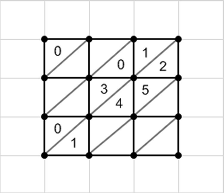 Figure 6: A simple grid-based mesh with triangles
Having a fixed topology which is based on a grid allows us to compute an index into a buffer as we did in the Filter method. As before, depending upon which corner or edge the vertex is on will change the number and indices of the surfaces which will be used in computing the normal. Let's take a look at an implementation which uses DirectX 10 to compute both surface and vertex normals on the GPU.
Implementing the Algorithm with DirectX 10
As with the filter method, the first thing we must do is define our vertex format.
struct MeshVertex
{
  D3DXVECTOR3 pos;
  unsigned i;
};
Rather than having a 2D position vector containing an x and z component, we've now got a full 3D position. The second parameter, an unsigned integer which I call i, will be used as the vertex's index. This index was unnecessary with the filter method because the x and z values combined could be used to compute where in the heightfield the vertex lied.
However, the arbitrary nature of vertices within a mesh makes it impossible to determine its relationship to other vertices based solely on its position. Thus, the index helps us to identify which normals are attached to any given vertex within the surface normal buffer. Next, we'll need to create a buffer and associated view resources. Unlike before, this buffer will be used store our surface normals rather than simple height values and will need to be both read from and written to by the geometry shader.
ID3D10Buffer* m_pNormalBufferSO;
ID3D10ShaderResourceView* m_pNormalBufferRVSO;
ID3D10EffectShaderResourceVariable* m_pSurfaceNormalsRV;
When creating our buffer we need to make sure that in addition to being bound as a shader resource, it is also bound as a stream output buffer so that it can be set as a stream output target.
void Heightfield::CreateShaderResources( int numSurfaces )
{
  // Create the non-streamed Shader Resources
  D3D10_BUFFER_DESC desc;
  D3D10_SHADER_RESOURCE_VIEW_DESC SRVDesc;

  // Create output normal buffer for the Stream Output
  ZeroMemory(&desc, sizeof(D3D10_BUFFER_DESC));
  ZeroMemory(&SRVDesc, sizeof(SRVDesc));
  desc.ByteWidth = numSurfaces * sizeof(D3DXVECTOR4);
  desc.Usage = D3D10_USAGE_DEFAULT;
  desc.BindFlags = D3D10_BIND_SHADER_RESOURCE | D3D10_BIND_STREAM_OUTPUT;
Next, we need to make sure that the buffer format is compatible with stream output stage and that it can be used as a stream output target. The only format I was able to successfully bind was DXGI_FORMAT_R32G32B32A32_FLOAT. I attempted to get it working with R32G32B32_FLOAT, a full 4 bytes smaller per buffer element, but the compiler claimed it was an incompatible type. This may suggest the stream output stage must treat each element as a full float4.
SRVDesc.Format = DXGI_FORMAT_R32G32B32A32_FLOAT;
SRVDesc.ViewDimension = D3D10_SRV_DIMENSION_BUFFER;
SRVDesc.Buffer.ElementWidth = numSurfaces;
m_pDevice->CreateBuffer(&desc, NULL, &m_pNormalBufferSO);
m_pDevice->CreateShaderResourceView(m_pNormalBufferSO, &SRVDesc, &m_pNormalBufferRVSO); }
After initializing all of our buffers and updating our mesh positions the next step is to draw our mesh. As before, we're going to create some local variables, set some necessary constants within our HLSL, and set the input layout, index buffer, and vertex buffers so that the input assembler knows how to construct and process our vertices for use by the vertex shader.
void Heightfield::Draw()
{
  int numRows = m_NumVertsDeep - 1;
  int numIndices = 2 * m_NumVertsWide;
  m_pNumVertsDeep->SetInt(m_NumVertsDeep);
  m_pNumVertsWide->SetInt(m_NumVertsWide);
  m_pMetersPerVertex->SetFloat(m_MetersPerVertex);
  m_pDevice->IASetPrimitiveTopology (D3D10_PRIMITIVE_TOPOLOGY_TRIANGLESTRIP);
  m_pDevice->IASetIndexBuffer(m_pIndexBuffer, DXGI_FORMAT_R32_UINT,0);
  UINT offset = 0; UINT stride = sizeof(MeshVertex);
  m_pDevice->IASetInputLayout(m_pMeshIL);
  m_pDevice->IASetVertexBuffers(0, 1, &m_pMeshVB, &stride, &offset);
Next, we get a chance to take a look at some new stuff. Here we're creating an array of ID3D10ShaderResourceView's containing a single element, NULL and setting it as the shader resource array of the Vertex Shader. We do this because we're using the same buffer for the stream output stage as input for our vertex shader. In order to do this we need to ensure that it's not still bound to the Vertex Shader from a previous pass when we attempt to write to it.
ID3D10ShaderResourceView* pViews[] = {NULL};
m_pDevice->VSSetShaderResources(0, 1, pViews);
Once we've cleared the shader resources attached to slot 0 we're going to set our surface normal buffer as the output for the stream output stage. This makes it so any vertices we add to the stream get stored within our buffer. Because we don't actually read from that buffer until the second pass, it's also fine to bind it to the Vertex Shader at this point.
m_pDevice->SOSetTargets(1, &m_pNormalBufferSO, &offset);
m_pSurfaceNormalsRV->SetResource(m_pNormalBufferRVSO);
Unlike the filter method, we take a few additional steps when calling draw here. First, because we're working with a technique which we know to have more than 1 pass we're going to be polite and actually ask the technique how many passes it has, and then iterate over both.
D3D10_TECHNIQUE_DESC desc;
m_pMeshWithNormalMapSOTech->GetDesc(&desc);

for(unsigned i = 0; i < numIndices; ++i)
{
  GetPassByIndex(i)->Apply(0);

  for (int j = 0; j < numIndices; j++)
  {
    DrawIndexed(numIndices, j * numIndices, 0 );
At the end of our first pass, after iterating over each of the rows in our mesh and drawing them, we need to make sure to clear the stream output targets so that in pass 1 we can use the surface normal buffer as an input to the vertex shader.
		m_pDevice->SOSetTargets(0, NULL, &offset);
	}
}
Next, we move on to the HLSL. While the technique declaration comes last within the HLSL file, I'm going to show it to you here first so you have a clear picture of how the technique is structured and how the 2 passes are broken down. In the first pass, pass P0, we're setting the vertex shader to contain a simple pass-through shader. All this shader does is take the input from the Input Assembler and pass it along to the Geometry Shader.
GeometryShader gsNormalBuffer = ConstructGSWithSO( CompileShader( gs_4_0, SurfaceNormalGS() ), "POSITION.xyzw" );

technique10 MeshWithNormalMapSOTech
{
  pass P0
  {
    SetVertexShader( CompileShader( vs_4_0, PassThroughVS() ) );
    SetGeometryShader( gsNormalBuffer );
    SetPixelShader( NULL );
  }
The next part of the declaration is assignment of the geometry shader. For clarity, the geometry shader is built before the pass declaration using the ConstructGSwithSO HLSL method. Of importance, the last parameter of the ConstructGSWithSO method is the output format of the primitives that are added to the streamed output. In our case, we're simply passing out a four-component position value, which, incidentally doesn't represent position, but represents our surface normal vectors. The final part of P0 is setting the pixel shader. Because P0 is strictly for computing our surface normals we're going to set the pixel shader to null. Once Pass 0 is complete, we render our mesh a second time using pass 1. In pass 1 we set a vertex shader which looks almost identical to the vertex shader we used for the filter method. The primary difference is that this vertex shader calls ComputeNormal instead of FilterNormal, resulting in a different approach to obtaining the vertex normal. Because Pass 1 is ultimately responsible for rendering our mesh to the screen we're going to leave our Geometry Shader null for this pass and instead provide a pixel shader. The pixel shader is just a standard shader for drawing a pixel at a given point using the color and position interpolated from the previous stage. Note we also enable depth buffering so that the mesh waves don't draw over themselves.
  pass P1
  {
    SetVertexShader( CompileShader( vs_4_0, RenderNormalMapScene() ) );
    SetGeometryShader( NULL );
    SetPixelShader( CompileShader( ps_4_0, RenderScenePS() ) );
    SetDepthStencilState( EnableDepth, 0 );
  }
}
Now let's take look at the most important of those shaders one at a time. The first item on the list is the Geometry Shader.
[maxvertexcount(1)]
void SurfaceNormalGS( triangle GS_INPUT input[3], inout PointStream PStream )
{
  GS_INPUT Output = (GS_INPUT)0;
  float3 edge1 = input[1].Position - input[0].Position;
  float3 edge2 = input[2].Position - input[0].Position;
  Output.Position.xyz = normalize( cross( edge2, edge1 ) );
  PStream.Append(Output);
}
Here we declare a simple geometry shader that takes as input a triangle and a point stream. Inside of the geometry shader we implement the first part of Gouraud's Smooth Shading algorithm by computing the cross-product of the provided triangle. Once we've done so, we normalize it, and then add it as a 4-component point to our point stream. This stream, which will be filled with float4 values, will serve as the surface normal buffer in the second pass. This leads us to the second part of Gouraud's Smooth shading algorithm. Rather than list the entire vertex shader here, let's focus on the code that actually does most of the work - ComputeNormal.
float3 ComputeNormal(uint index)
{
  float3 normal = 0.0;
  int topVertex = g_NumVertsDeep - 1;
  int rightVertex = g_NumVertsWide - 1;
  int normalsPerRow = rightVertex * 2;
  int numRows = topVertex;
  float top = normalsPerRow * (numRows - 1);
  int x = index % g_NumVertsWide;
  int z = index / g_NumVertsWide;

  // Bottom
  if(z == 0)
  {
    if(x == 0)
    {
      float3 normal0 = g_SurfaceNormals.Load(int2( 0, 0 ));
      float3 normal1 = g_SurfaceNormals.Load(int2( 1, 0 ));
      normal = normal0 + normal1;
    }
    else if(x == rightVertex)
    {
      index = (normalsPerRow - 1);
      normal = g_SurfaceNormals.Load(int2( index, 0 ));
    }
    else
    {
      index = (2 * x);
      normal = g_SurfaceNormals.Load(int2( index-1, 0 )) + g_SurfaceNormals.Load(int2( index, 0 )) + g_SurfaceNormals.Load(int2( index+1, 0 ));
    }
  }
  // Top
  else if(z == topVertex)
  {
    if(x == 0)
    {
      normal = g_SurfaceNormals.Load(int2( top, 0 ));
    }
    else if(x == rightVertex)
    {
      index = (normalsPerRow * numRows) - 1;
      normal = g_SurfaceNormals.Load(int2( index, 0 )) + g_SurfaceNormals.Load(int2( index-1, 0 ));
    }
    else
    {
      index = top + (2 * x);
      normal = g_SurfaceNormals.Load(int2( index-2, 0)) + g_SurfaceNormals.Load(int2( index, 0)) + g_SurfaceNormals.Load(int2( index-1, 0));
    }
  }
  // Middle
  else
  {
    if(x == 0)
    {
      int index1 = z * normalsPerRow;
      int index2 = index1 - normalsPerRow;
      normal = g_SurfaceNormals.Load(int2( index1, 0 )) + g_SurfaceNormals.Load(int2( index1+1, 0 )) + g_SurfaceNormals.Load(int2( index2, 0 ));
    }
    else if(x == rightVertex)
    {
      int index1 = (z + 1) * normalsPerRow - 1;
      int index2 = index1 - normalsPerRow;
      normal = g_SurfaceNormals.Load(int2( index1, 0 )) + g_SurfaceNormals.Load(int2( index2, 0 )) + g_SurfaceNormals.Load(int2( index2-1, 0 ));
    }
    else
    {
      int index1 = (z * normalsPerRow) + (2 * x);
      int index2 = index1 - normalsPerRow;
      normal = g_SurfaceNormals.Load(int2( index1-1, 0 )) + g_SurfaceNormals.Load(int2( index1, 0 )) + g_SurfaceNormals.Load(int2( index1+1, 0 )) + g_SurfaceNormals.Load(int2( index2-2, 0 )) + g_SurfaceNormals.Load(int2( index2-1, 0 )) + g_SurfaceNormals.Load(int2( index2, 0 ));
    }
  }

  return normal;
}
As with the filter algorithm for heightmap based terrain, the ComputeNormal method performs a series of checks to determine whether the vertex is on the left, middle, or right edge, and whether it's on the bottom, center, or top edge of the grid. Depending on the answer, between one and six surface normals are sampled from the buffer and then summed together. The result is then returned to the main entry function for the vertex shader, where it is normalized, and used in computing the final color of the Vertex.
Conclusion
The code snippets contained within this article are based on the accompanying demo which is written in C++ using DirectX 10 and HLSL, and contains not only the algorithms detailed here but also the two remaining methods for computing vertex normals for a grid-based mesh. That is, it computes the Surface and Vertex normals on the CPU, and also computes the Surface normals on the CPU while using the GPU for the Vertex Normals. Please make sure to download those files, run the demo for yourself, and evaluate the remaining source code. You can then perform a personal comparison of the performance afforded to you by each method. For an idea of what the demo looks like, refer to Figure 7.
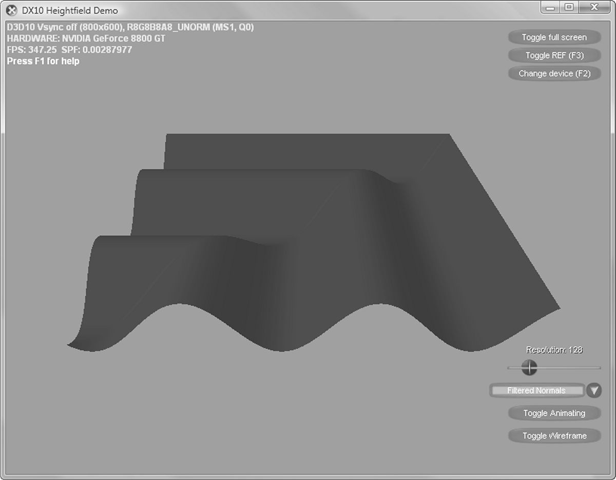 Figure 7: A screenshot of the demo program for this article
As the demo uses DirectX 10 and SM 4.0, you will need a computer running Windows Vista and a compatible video card with the most up-to-date DirectX SDK and drivers in order to successfully run the application. The limited documentation for the demo can be displayed within the application by pressing the F1 key. Additionally, on the lower right-hand corner of the screen there are four controls which can be used to configure the demonstration. The resolution slider identifies the number of vertices across and deep the terrain sample will be. The slider ranges from 17 to 512. Below the Resolution Slider is a combo box which allows the user to select from one of the 4 different methods of implementation within the demo: "Filtered Normals", "CPU Normals", "GPU Normals", and "Streamed Normals". Below the normal mode combo boxes are two buttons labeled "Toggle Animation" and "Toggle wireframe". No surprise, these either toggle on/off the animation or toggle on/off wireframe mode, respectively.
References
"Normal Computations for Heightfield Lighting", Jeromy Walsh (@JWalsh), 2005, GameDev.net