Introduction
Backpropagation
The backpropagation algorithm is perhaps the most widely used training algorithm for multi-layered feedforward networks. However, many people find it quite difficult to construct multilayer feedforward networks and training algorithms from scratch, whether it be because of the difficulty of the math (which can seem misleading at first glance of all the derivations) or the difficulty involved with the actual coding of the network and training algorithm. Hopefully after you have read this guide you'll walk away knowing more about the backpropagation algorithm than you ever did before. Before continuing further on in this tutorial you might want to check out James' introductory essay on neural networks.

Summary
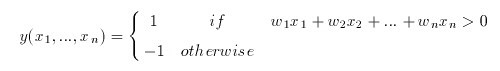
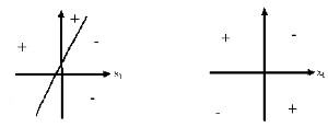
The problem with the perceptron is that it cannot express non-linear decisions. The perceptron is basically a linear threshold device which returns a certain value, 1 for example, if the dot product of the input vector and the associated weight vector plus the bias surpasses the threshold, and another value, -1 for example, if the threshold is not reached.
When the dot product of the input vector and the associated weight vector plus the bias f(x1,x2,..,xn)=w1x1+w2x2+...wnxn+wb=threshold, is graphed in the x1,x2,...,xn coordinate plane/space one will notice that it is obviously linear. More than that however, this function separates this space into two categories. All the input vectors that will give a (f(x1,x2,..,xn)=w1x1+w2x2+...wnxn+wb) value greater than the threshold are separated into one space, and those that will not will be separated into another (see figure).

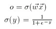
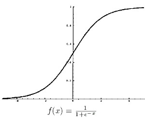
The obvious problem with this model then is, what if the decision cannot be linearly separated? The failure of the perceptron to learn the XOR network and to distinguish between even and odd almost led to the demise of faith in neural network research. The solution came however, with the development of neuron models that applied a sigmoid function to the weighted sum (w1x1+w2x2+...wnxn+wb) to make the activation of the neuron non-linear, scaled and differentiable (continuous). An example of a commonly used sigmoid function is the logistic function given by o(y)=1/(1+e^(-y)), where y=w1x1+w2x2+...wnxn+wb. When these "sigmoid units" are arranged layer by layer, with each layer downstream another layer acting as the input vector etc. the multilayer feedforward network is created.
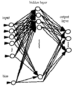
Multilayer feedforward networks normally consist of three or four layers, there is always one input layer and one output layer and usually one hidden layer, although in some classification problems two hidden layers may be necessary, this case is rare however. The term input layer neurons are a misnomer, no sigmoid unit is applied to the value of each of these neurons. Their raw values are fed into the layer downstream the input layer (the hidden layer). Once the neurons for the hidden layer are computed, their activations are then fed downstream to the next layer, until all the activations eventually reach the output layer, in which each output layer neuron is associated with a specific classification category. In a fully connected multilayer feedforward network, each neuron in one layer is connected by a weight to every neuron in the layer downstream it. A bias is also associated with each of these weighted sums. Thus in computing the value of each neuron in the hidden and output layers one must first take the sum of the weighted sums and the bias and then apply f(sum) (the sigmoid function) to calculate the neuron's activation.

How then does the network learn the problem at hand? By modifying the all the weights of course. If you know calculus then you might have already guessed that by taking the partial derivative of the error of the network with respect to each weight we will learn a little about the direction the error of the network is moving. In fact, if we take negative this derivative (i.e. the rate change of the error as the value of the weight increases) and then proceed to add it to the weight, the error will decrease until it reaches a local minima. This makes sense because if the derivative is positive, this tells us that the error is increasing when the weight is increasing, the obvious thing to do then is to add a negative value to the weight and vice versa if the derivative is negative. The actual derivation will be covered later. Because the taking of these partial derivatives and then applying them to each of the weights takes place starting from the output layer to hidden layer weights, then the hidden layer to input layer weights, (as it turns out this is neccessary since changing these set of weights requires that we know the partial derivatives calculated in the layer downstream) this algorithm has been called the "back propagation algorithm".

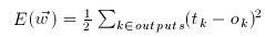
How is the error of the network computed? In most classification networks the output neuron that achieves the highest activation is what the network classifies the input vector to be. For example if we wanted to train our network to recognize 7x7 binary images of the numbers 0 through 9, we would expect our network to have 10 output neurons, which each output neuron corresponding to one number. Thus if the first output neuron is most activated, the network classifies the image (which had been converted to a input vector and fed into the network) as "0". For the second neuron "1", etc. In calculating the error we create a target vector consisting of the expected outputs. For example, for the image of the number 7, we would want the eigth output neuron to have an activation of 1.0 (the maximum for a sigmoid unit) and for all other output neurons to achieve an activation of 0.0. Now starting from the first output neuron calculate the squared error by squaring the difference between the target value (expected value for the output neuron) and the actual output value and end at the tenth output neuron. Take the average of all these squared errors and you have the network error. The error is squared as to make the derivative easier.
Once the error is computed, the weights can be updated one by one. This process continues from image to image until the network is finally able to recognize all the images in the training set.
Training
Recall that training basically involves feeding training samples as input vectors through a neural network, calculating the error of the output layer, and then adjusting the weights of the network to minimize the error. Each "training epoch" involves one exposure of the network to a training sample from the training set, and adjustment of each of the weights of the network once layer by layer. Selection of training samples from the training set may be random (I would recommend this method escpecially if the training set is particularly small), or selection can simply involve going through each training sample in order.
Training can stop when the network error dips below a particular error threshold (Up to you, a threshold of .001 squared error is good. This varies from problem to problem, in some cases you may never even get .001 squared error or less). It is important to note however that excessive training can have damaging results in such problems as pattern recognition. The network may become too adapted in learning the samples from the training set, and thus may be unable to accurately classify samples outside of the training set. For example, if we over trained a network with a training set consisting of sound samples of the words "dog" and "cog", the network may become unable to recognize the word "dog" or "cog" said by a unusual voice unfamiliar to the sound samples in the training set. When this happens we can either include these samples in the training set and retrain, or we can set a more lenient error threshold.
These "outside" samples make up the "validation" set. This is how we assess our network's performance. We can not expect to assess network performance based solely on the success of the network in learning an isolated training set. Tests must be done to confirm that the network is also capable of classifying samples outside of the training set.
Backpropagation Algorithm
The first step is to feed the input vector through the network and compute every unit in the network. Recall that this is done by computing the weighting sum coming into the unit and then applying the sigmoid function. The 'x' vector is the activation of the previous layer.

The second step is to compute the squared error of the network. Recall that this is done by taking the sum of the squared error of every unit in the output layer. The target vector involved is associated with the training sample (the input vector).

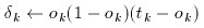
The third step is to calculate the error term of each output unit, indicated below as 'delta'.

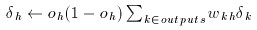
The fourth step is to calculate the error term of each of the hidden units.

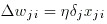
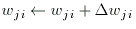
The fifth step is to compute the weight deltas. 'Eta' here is the learning rate. A low learning rate can ensure more stable convergence. A high learning rate can speed up convergence in some cases.

The final step is to add the weight deltas to each of the weights. I prefer adjusting the weights one layer at a time. This method involves recomputing the network error before the next weight layer error terms are computed.


Very interesting and informative article. Thanks for the information you shared.