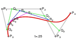
This is meant as an intermediate guide to Bezier curves. I'm assuming you've all read about Bezier curves and the Bernstein basis functions and have a general idea about how it all works. This is meant as the next level up and some ways to implement them in practical code. This isn't meant as a thorough exploration of the mathematics, but as a jump-off point. I'm sure others here know more than I do, but I'd like to introduce some things here that can be helpful to those who want to delve into this topic.

The Story So Far...

Bernstein Basis Polynomials

To quickly sum things up, Bezier (pronounced [be.zje]) curves use the Bernstein basis functions multiplied by control points to create a curve. A Bernstein basis function takes the form \( b_{i,n}(t) = \binom{n}{i}t^i(1-t)^{n-i} \), where i is the ith basis function and n is the degree of the Bernstein basis. The basis function form a partition of unity, which means that for any parameter value between 0 and 1, \( \sum_{i=0}^n b_i(t) = 1 \). A Bernstein polynomial is simply where the basis functions are multiplied by coefficients and summed: \( B_{i,n}(t) = \sum_{i=0}^n c_ib_{i,n}(t) = \sum_{i=0}^n c_i \binom{n}{i} t^i (1-t)^{n-i} \), where c is the coefficient for the ith term. This polynomial is a parametric curve. To clarify, the sum in the Bernstein polynomial doesn't just add to 1 because of the coefficients.

Bezier Curves

You've probably seen this equation so many times you know it by heart: \[ C(t) = \sum_{i=0}^n \binom{n}{i} (1-t)^{n-i} t^i P_i \] N-dimensional Bezier curves can be expressed as N Bernstein polynomials where the coefficients of the Bernstein polynomials are the control points in a certain dimension. For example, a 2D Bezier curve can be expressed as 2 Bernstein polynomials, one for the x-direction and one for the y-direction: \[ \begin{cases} x(t) &= \sum_{i=0}^n \binom{n}{i} (1-t)^{n-i} t^i x_i \\ y(t) &= \sum_{i=0}^n \binom{n}{i} (1-t)^{n-i} t^i y_i \\ \end{cases} \] The control points are given as \( P_i = (x_i,y_i) \). There are n+1 control points for a degree-n Bezier curve. 3D and 4D curves can be expressed in this same fashion. Bezier curves can have any bounds on the t-parameter, but unless specified it can be assumed that it only varies from 0 to 1. Note: if the interval isn't between 0 and 1, the curve definition takes on a slightly modified form: \[ C_{[t_0,t_1]}(t) = \sum_{i=0}^n \binom{n}{i} \left ( \frac{t_1-t}{t_1-t_0} \right )^{n-i} \left ( \frac{t-t_0}{t_1-t_0} \right )^{i} \] Bezier curves allow the user to intuitively control the shape of the curve. As the control points move in a certain direction, the curve moves in that direction too. We can gain some additional control of our curve by creating rational Bezier curves.

The Cool, New Stuff

Bezier Curve Evaluation

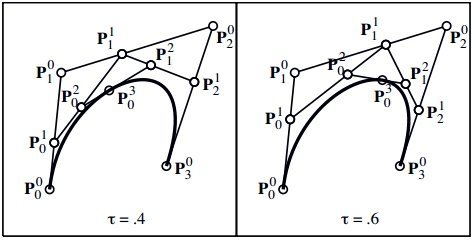
Before we get too far into rational Beziers, let's go over evaluation of Bezier curves. We could just do the simple evaluation of Bezier curves and get our answer. Let's say we're not so naive and used the recurrence relation for the binomial coefficient (if you're not familiar with the binomial coefficient, read the Wikipedia article): \( \binom{n}{i} = \frac{n-i+1}{i} \binom{n}{i-1} \). For 3D curves, the pseudocode might go like this: function evaluate(double t) { x = 0, y = 0, z = 0; nChooseI = 1; for(int i=0;i<controlpoints.length;i++) { u = pow(t,i); uComp = pow(1-t,i); p = u * uComp; if(i != 0) { nChooseI *= (n-i+1)/i; } x += nChooseI * controlpoints.x * p; y += nChooseI * controlpoints.y * p; z += nChooseI * controlpoints.z * p; } return x,y,z; } Even with all of our tricks, we're still computing the power terms on each loop. So what can we do to get faster? Turns out there's 4 simple methods for quick evaluation:

1. Use the de Casteljau method.
2. Use a modified form of Horner's algorithm.
3. If you want to compute the whole curve quickly, use a forward difference table.
4. **Construct a set of matrices and multiply for evaluation.

de Casteljau Method The de Casteljau method is a technique that takes advantage of the nature of the Bernstein basis functions. To start, let's say the t-parameter of a Bezier curve is between 0 and 1. If that curve is a degree-1, it represents a line between the 2 control points. If t=0, the evaluated point is P0; if t=1, the evaluated point is P1. If t=0.5, the point is halfway between the control points. The t-parameter tells us how far to go between P0 and P1. The Bezier curve takes the form \( P(t) =(1-t)P_0+tP_1 \). This is how linear interpolation is done. Now let's say we had a degree-2 curve. The Bernstein basis functions would arise if we linearly interpolated between P0 and P1, between P1 and P2, then linearly interpolated between those 2 linearly interpolated points. The t-parameter would tell us how far to interpolate at each step. Mathematically, it would look something like this: \[ \begin{align} P(t)&=[(1-t)P_0+tP_1](1-t)+[(1-t)P_1+tP_2]t \\ P(t)&=(1-t)^2P_0+t(1-t)P_1+t(1-t)P_1+t^2P_2 \\ P(t)&=(1-t)^2P_0+2t(1-t)P_1+t^2P_2 \\ \end{align} \] The Wikipedia article shows how the curve is constructed in this manner. Since the degree for this is 2, 2 linear interpolations are done. The higher order the polynomial, the more linear interpolations are done. This is precisely how the de Casteljau method works. Mathematically, the de Casteljau method looks like this:

\[ P_i^j = (1-\tau)P_i^{j-1}+\tau P_{i+1}^{j-1}; j=1,\dots,n; i=0,\dots,n-j \] The tau must be between 0 and 1. Incidentally, the de Casteljau method is useful for breaking up a Bezier curve into 2 Bezier curves. In the formula above, the points \( P_0^0,P_0^1,\dots,P_0^n \) are the control points for the Bezier curve on the interval \( (0, \tau) \) of the original curve, and the points \( P_0^n,P_1^{n-1},\dots,P_n^0 \) are the control points for the Bezier curve on the interval \( (\tau, 1) \) of the original curve. The de Casteljau method is really nice because it's numerically stable, meaning that repeated use of it won't introduce numerical error into your calculations and throw them off. Modified Horner's Method The following code is the modified version of Horner's algorithm for quick evaluation. It takes advantage of the recurrence relation for the binomial coefficient as well as implements the nested multiplication like the classic Horner's algorithm: function eval_horner(t) { u = 1 - t; bc = 1; tn = 1; tmp = controlpoints[0] * u; for(int i = 1; i < n; i++) { tn *= t; bc *= (n-i+1)/i; tmp = (tmp + tn * bc * controlpoints) * u; } return (tmp + tn * t * controlpoints[n]); } Forward Differencing If you're evaluating a curve at evenly-spaced intervals, forward differencing is the fastest method, even faster than Horner's algorithm. For a degree-n polynomial, Horner's algorithm requires n multiplies and n adds. However, the forward differencing method only requires n additions, after a small initialization (which we could use Horner's algorithm for). There is a derivation for this method that I won't show here, but you can try this out and evaluate with Horner's and compare the methods. This method requires n+1 curve evaluations to initiate the forward differencing. The easiest explanation of the method is to demonstrate it. Let's say that we had a degree-4 polynomial and the first 5 evaluations were: f(i)=1, f(i+1)=3, f(i+2)=2, f(i+3)=5, and f(i+4)=4. We build a table by subtracting f(i+1)-f(i), putting that value in the next row, and so on, like the following: \[ \begin{matrix} t & t_i & t_{i+1} & t_{i+2} & t_{i+3} & t_{i+4} & t_{i+5} & t_{i+6} & t_{i+7} \\ f(t) & 1 & 3 & 2 & 5 & 4 & & & \\ \delta_1(t) & 2 & -1 & 3 & -1 & & & & \\ \delta_2(t) & -3 & 4 & -4 & & & & & \\ \delta_3(t) & 7 & -8 & & & & & & \\ \delta_4(t) & -15 & & & & & & & \\ \end{matrix} \] The method states that the number in the last row, -15 in this case, will stay constant for every column in that row. That means that if we put -15 in the next column, then add -15 to the number above it (-8), store that value in the next column on that row, and do this until we reach the value row, we can compute the value for f(i+5). Repeat for f(i+6), and all successive values for f(t). It would look something like this: \[ \begin{matrix} t & t_i & t_{i+1} & t_{i+2} & t_{i+3} & t_{i+4} & t_{i+5} & t_{i+6} & t_{i+7} \\ f(t) & 1 & 3 & 2 & 5 & 4 & -24 & -117 & -328 \\ \delta_1(t) & 2 & -1 & 3 & -1 & -28 & -93 & -211 & \\ \delta_2(t) & -3 & 4 & -4 & -27 & -65 & -118 & & \\ \delta_3(t) & 7 & -8 & -23 & -38 & -53 & & & \\ \delta_4(t) & -15 & -15 & -15 & -15 & & & & \\ \end{matrix} \] This method is fast, but it's numerically unstable. This means that eventually, over the course of the forward difference, errors creep in and throw off the computation. This means a lot to the CAD world, but for rendering forward differencing is usually sufficient. Matrix Evaluation There is a matrix evaluation that can be quick as well, but that discussion is better suited to the discussion on Bezier surfaces. See the Bezier surface article here.

Rational Bezier Curves

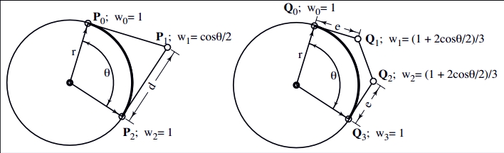
A rational Bezier curve adds a weight to each control point. As the weight increases, the curve bends toward that control point. The formulation for a rational Bezier curve is given by: \[ B(t) = \frac{\sum_{i=0}^n w_i \, P_i \, b_i(t)}{\sum_{i=0}^n w_i \, b_i(t)} = \left ( \frac{\sum_{i=0}^n w_i \, x_i \, b_i(t)}{\sum_{i=0}^n w_i \, b_i(t)}, \frac{\sum_{i=0}^n w_i \, y_i \, b_i(t)}{\sum_{i=0}^n w_i \, b_i(t)}, \frac{\sum_{i=0}^n w_i \, z_i \, b_i(t)}{\sum_{i=0}^n w_i \, b_i(t)} \right ) \] As you can see, if all the weights are 1, then the curve becomes a normal Bezier curve. Rational Bezier curves help us because:

1. Rational Bezier curves can represent conic sections exactly.
2. Perspective projections of Bezier curves are rational Bezier curves.
3. The weights allow for additional control of the curve.
4. Reparameterization of the curve is accomplished by changing the weights in a certain fashion (which I won't get into here).

Rational curves allow us to represent circular arcs (since a circle is a conic section). The image below shows what this would look like:

A degree-2 rational Bezier curve can represent an arc. The control points P0 and P2 must be on the circle, but the control point P1 is at the intersection of the extended tangent lines of the circle at P0 and P2. The weights of the control points P0 and P2 are 1, but the weight of control point P1 is cos(theta)/2, where theta is the angle of the arc. A degree-3 (cubic) Bezier curve can also represent a circular arc. Like in the degree-2 case, the endpoints P0 and P3 must be on the circle, but P1 and P2 must lie on the extended tangent lines of the circle at P0 and P3, respectively. The distance that P1 and P2 must be from P0 and P3, respectively, is given by the equation \( e = \frac{2\sin{\theta / 2}}{1+2\cos{\theta / 2}} \).

Rational Bezier Curves as 4D Bezier Curves

Yup, just like the title says, rational Bezier curves can be represented as 4D Bezier curves. I know some of you might be scratching your head and clicking to a new page, but let me explain. If we create a mapping from a 4D curve to our 3D rational curve, we could do some normal Bezier curve evaluation using the algorithms above and not have to modify them. The mapping is simple: if in 3D we have (x,y,z) and weight w, then in 4D we can express it as (X,Y,Z,W) = (x*w, y*w, z*w, w). That means that the conversion from 4D to 3D is as simple as division. This does create weird equalities, such as point (x,y,z) in 3D maps to multiple points in 4D, such as (2x, 2y, 2z, 2), (3x, 3y, 3z, 3), and so on. For our purposes, this is just fine, so just something to note. This mapping works for rational curves because, as we stated above, when all the weights equal 1, then the rational curve is identical to a normal Bezier curve. By elevating the problem to a higher dimension, we gain a lot of computational simplicity. (As an aside, a similar mapping can be made from 2D rational Bezier curves to 3D normal Bezier curves, and you can picture the 3D-to-2D mapping as the projection of the 3D curve onto the plane z=1.) In 4D, that means a 3D rational Bezier curve takes the following form: \[ \begin{cases} X(t)&=x_iw_ib_i(t)\\ Y(t)&=y_iw_ib_i(t)\\ Z(t)&=z_iw_ib_i(t)\\ W(t)&=w_ib_i(t)\\ \end{cases} \] If you look at the top 3 equations, they're identical to the expanded numerator of the rational Bezier definition. If you notice, the bottom equation is identical to the denominator of the rational Bezier. This means that if we want to compute a 3D rational Bezier curve, we can simply elevate it to 4D space, do one more additional computation in our curve evaluation, then just do the perspective divide of the point back to 3D. In fact, we can elevate all our regular Bezier curves into 4D by making the weights 1, and then just do perspective divide to get the point back to 3D. NOTE: Elevating rational Bezier curves makes evaluation and a few things easier, but it doesn't make all problems easier. For example, if you want the derivative of a rational Bezier curve, you can't just elevate it to 4D and then take the derivative and then project back. Derivatives of rational Bezier curves involve the quotient rule from calculus, something that a higher dimensionality doesn't simplify.

Conclusion

One of the primary difficulties with the Bezier formulation is that each control point influences the entire curve. Also, the number of control points is directly tied to the degree of the resulting Bernstein polynomials. Thus, a Bezier curve with 6 control points yields a 5th degree polynomial. Evaluating higher degree polynomials takes extra computation time (even with Horner's algorithm, so we want to avoid having high degree polynomials if possible. These problems have been overcome by B-splines. B-splines aren't much harder to understand once you get Bezier curves down. In the future, if there's enough response here, I'll add a basic introduction to B-splines and easy ways to generate them (not necessarily computationally efficient) and do them by hand too.

Article Updates

04 Aug 2013: Updated equations to use MathJax 05 Jun 2013: Fixed some typographical errors 28 May 2013: Initial release

References

A lot of the information here was taught to me by Dr. Thomas Sederberg (associate dean at Brigham Young University, inventor of the T-splines technology, and recipient of the 2006 ACM SIGGRAPH Computer Graphics Achievement Award). The rest came from my own study of relevant literature.