Introduction
Verlet integration is a nifty method for numerically integrating the equations of motion (typically linear, though you can use the same idea for rotational). It is a finite difference method that's popular with the Molecular Dynamics people. Actually, it comes in three flavors: the basic Position, the Leapfrog and the Velocity versions. We will be discussing the Position Verlet algorithm in this paper. It has the benefit of being quite stable, especially in the face of enforced boundary conditions (there is no explicit velocity term with which the position term can get out of sync). It is also very fast to compute (almost as fast as Euler integration), and under the right conditions it is 4[sup]th[/sup] order accurate (by comparison, the Euler method is only 1[sup]st[/sup] order accurate, and the second order Runge-Kutta method is only 2[sup]nd[/sup] order accurate [go figure]).

The disadvantages of the Verlet method are that it handles changing time steps badly, it is not a self-starter (it requires 2 steps to get going, so initial conditions are crucial), and it is unclear from the formulation how it handles changing accelerations. In this paper we will discuss all of these shortcomings, and see how to minimize their impact. The modified Verlet integrator is referred to as the Time-Corrected Verlet (TCV) and is shown below with its original counterpart. The computations used to generate the graphs for this paper are included in this Excel file.

Original Verlet:
x[sub]i+1[/sub] = x[sub]i[/sub] + (x[sub]i[/sub] - x[sub]i-1[/sub]) [sub]+[/sub] a * dt * dt

Time-Corrected Verlet:
x[sub]i+1[/sub] = x[sub]i[/sub] + (x[sub]i[/sub] - x[sub]i-1)[/sub] * (dt[sub]i[/sub] / dt[sub]i-1[/sub]) + a * dt[sub]i[/sub] * dt[sub]i[/sub]

To see why the TCV is an improvement, we need to see the math behind the original Verlet method.


Math
In this paper we will be talking exclusively about point masses, which are acted on by forces. Well, we all know about Newton's little equation: Force=d(Momentum)/dt. Momentum=mass*velocity and for non-relativistic speeds the mass is constant, removing our need for the chain rule, and yielding our familiar F=ma. So if all the forces acting on the point mass are summed (the vector F), then scaled by (1.0/m) we have the acceleration (a) of the point mass. Since we know how to go from force to acceleration, we will be starting from the acceleration term to keep the math less cluttered. In actual applications you will almost always be summing forces, then converting to accelerations.

Most of the graphs presented in this paper include the matching Euler simulation, just for reference. The Euler algorithm is extremely simple, and it will not be derived here. However, the equations are included below for your reference (order is important):

v = v + a * dt
x = x + v * dt

There is a more accurate version, but it is not strictly the Euler method, so it will not be used for this paper. However it does give 2[sup]nd[/sup] order accurate results, instead of merely 1[sup]st[/sup] order:

x = x + v * dt + 0.5 * a * dt * dt
v = v + a * dt

Please note that there is a faster way to derive the Verlet method's math* than what will be shown here, however it does not provide the insight needed to overcome the issues mentioned in the introduction. So we'll start from a few basic principles: a=dv/dt, and v=dx/dt. So for any given point mass, if we know the current position, velocity and acceleration (the acceleration must be constant over the given time step), we can compute exactly where it will be after the time step (dt) has elapsed.

(1) x[sub]i+1[/sub] = x[sub]i[/sub] + v[sub]i[/sub] * dt[sub]i[/sub] + 0.5 * a[sub]i[/sub] * dt[sub]i[/sub] * dt[sub]i[/sub]

or

(1a) x[sub]i+1[/sub] - x[sub]i[/sub] = v[sub]i[/sub] * dt[sub]i[/sub] + 0.5 * a[sub]i[/sub] * dt[sub]i[/sub] * dt[sub]i[/sub]

Now, if we wanted that equation formulated without the velocity term, we could replace it with some other known state variable, such as the position x. But since we don't know x[sub]i+1[/sub] yet, we shift the whole equation back a step:

(2) x[sub]i[/sub] - x[sub]i-1[/sub] = v[sub]i-1[/sub] * dt[sub]i-1[/sub] + 0.5 * a[sub]i-1[/sub] * dt[sub]i-1[/sub] * dt[sub]i-1[/sub]

and we can use simple integration to see that:

(3) v[sub]i[/sub] = v[sub]i-1[/sub] + a[sub]i-1[/sub] * dt[sub]i-1[/sub]

or

(3a) v[sub]i-1[/sub] = v[sub]i[/sub] - a[sub]i-1[/sub] * dt[sub]i-1[/sub]

and we substitute that into equation (2):

(4) x[sub]i[/sub] - x[sub]i-1[/sub] = (v[sub]i[/sub] - a[sub]i-1[/sub] * dt[sub]i-1[/sub]) * dt[sub]i-1[/sub] + 0.5 * a[sub]i-1[/sub] * dt[sub]i-1[/sub] * dt[sub]i-1[/sub]

or

(4a) x[sub]i[/sub] - x[sub]i-1[/sub] = v[sub]i[/sub] * dt[sub]i-1[/sub] - 0.5 * a[sub]i-1[/sub] * dt[sub]i-1[/sub] * dt[sub]i-1[/sub]

For this next step we need to make a big assumption, the importance of which will be seen later: If we assume that neither the acceleration nor the time step vary between steps (i.e. that a[sub]i-1[/sub] = a[sub]i[/sub] = a and that dt[sub]i-1[/sub] = dt[sub]i[/sub] = dt) then we note that:

(5) x[sub]i[/sub] - x[sub]i-1 +[/sub] a * dt * dt = v[sub]i[/sub] * dt - 0.5 * a * dt * dt + a * dt * dt

or

(5a) x[sub]i[/sub] - x[sub]i-1 +[/sub] a * dt * dt = v[sub]i[/sub] * dt + 0.5 * a * dt * dt

You'll notice that the right hand side of equation (5a) is exactly the last half of equation (1), so we can work the modified equation (5a) back into equation (1):

(6) x[sub]i+1[/sub] = x[sub]i[/sub] + (x[sub]i[/sub] - x[sub]i-1[/sub]) [sub]+[/sub] a * dt * dt

and there you have the traditional Verlet Position integration method.


Fundamental Problems
As you saw from the derivation's step (5), the two criteria needed to make the Verlet algorithm exact are constant acceleration and constant time step. For most practical cases we cannot guarantee either of these criteria. Of course, there are some simple cases where both criteria will be met. For example, simple projectile physics simulated by a physics engine which uses fixed time steps will yield perfect results. As soon as you add friction, springs or constraints of any kind you nullify the constant acceleration criterion, and adapting your time step to your game's framerate will nullify the constant time step criterion.

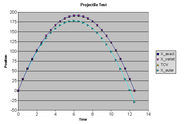
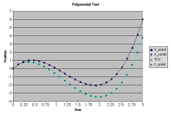
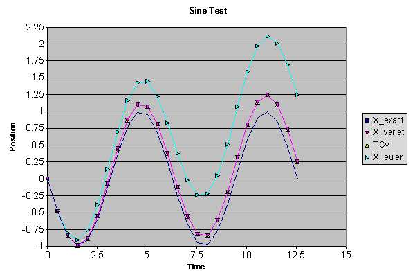
I am not going to address the constant acceleration criterion, mainly because explicit integrators (such as this one) must assume the constant acceleration principle, which is violated the instant you start simulating a complex system. Take the example of a point mass connected to a spring: as soon as it starts to move, the spring force, and thus the acceleration, changes. Even equation (1) required that the acceleration be constant throughout a time step. The error introduced by assuming that a[sub]i-1 =[/sub] a[sub]i[/sub] is actually implicit in our choosing an explicit scheme without knowing how the acceleration changes. We are effectively setting d(a)/dt (a.k.a. the "jerk") to 0.0. The other reason I will ignore this issue is that, empirically, the standard Verlet method already handles changing accelerations better than the Euler method (or even the improved variation on the Euler method), as long as the time step is fixed. Note that the Time-Corrected Verlet will be identical to the original Verlet when the time step is fixed. Observe the following graphs:







The error introduced by the constant time step assumption is something that can be easily ameliorated. This will be shown in the section entitled "A Simple Time-Correction Scheme".


Implementation Problems
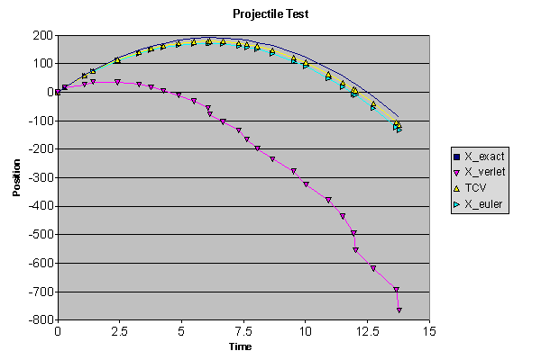
A large source of inaccuracy when using the Verlet scheme stems from the improper specification of initial conditions. Looking at equation (6) and trying to fit it into the form of equation (1) (which may be more familiar) may yield (improper) reasoning like this: the first (x[sub]i[/sub]) term is the position contribution, the second (x[sub]i[/sub] - x[sub]i-1[/sub]) term is basically the velocity contribution, and the (a * dt * dt) term is clearly the acceleration contribution. So when simulating the traditional projectile path, setting x[sub]0[/sub] = 0.0, and x[sub]-1[/sub]=x[sub]0[/sub] - v[sub]0[/sub] * dt[sub]0[/sub], and running the simulation from there will give the wrong results, as can be seen in the following graph:



This is because both the second and third terms include acceleration information. So, when setting the current state explicitly (i.e. the position and velocity initial conditions), remember to use equation (2). Shooting simulations depend upon starting with accurate initial conditions. The larger the initial time step, the less accurate your computed initial state will be if you do not use equation (2).


A Simple Time-Correction Scheme
The remaining fundamental problem with the Verlet integration method lies with its assumption of a constant time step. The (x[sub]i[/sub] - x[sub]i-1[/sub]) term from equation (4a) is the portion of the equation which is dependent on the constant acceleration and constant time step assumptions. It has been explained (OK, hand-waved away) why the usage of the last time step's acceleration will not be corrected, but we still have the problem of dt[sub]i-1[/sub] being stale information. Rewriting equation (4) yet again, we see that:

(4b) x[sub]i[/sub] - x[sub]i-1[/sub] = (v[sub]i[/sub] - 0.5 * a[sub]i-1[/sub] * dt[sub]i-1[/sub]) * dt[sub]i-1[/sub]

so taking the easy way out and ignoring the dt[sub]i-1[/sub] linked with the acceleration, I can swap out the old dt[sub]i-1[/sub] for my new dt[sub]i[/sub] by multiplying (4b) by (dt[sub]i[/sub] / dt[sub]i-1[/sub]). Plugging all of this in yields my final form of the Time-Corrected Verlet integration method:

(7) x[sub]i+1[/sub] = x[sub]i[/sub] + (x[sub]i[/sub] - x[sub]i-1)[/sub] * (dt[sub]i[/sub] / dt[sub]i-1[/sub]) + a * dt[sub]i[/sub] * dt[sub]i[/sub]

You will notice that when the last frame's time step equals the current frame's time step, the modifier term becomes 1.0, yielding the traditional form of the Verlet equation. As an optimization note, only one value needs to be stored per frame, as the dt was constant for all points in the last frame. So the term (dt[sub]i[/sub] / dt[sub]i-1[/sub]) can be computed once per frame and stored in a variable. At the end of the Verlet update subroutine simply store the current frame's dt as old_dt. Likewise, dt[sub]i[/sub] * dt[sub]i[/sub] can be computed once and stored in a variable, saving a multiplication.

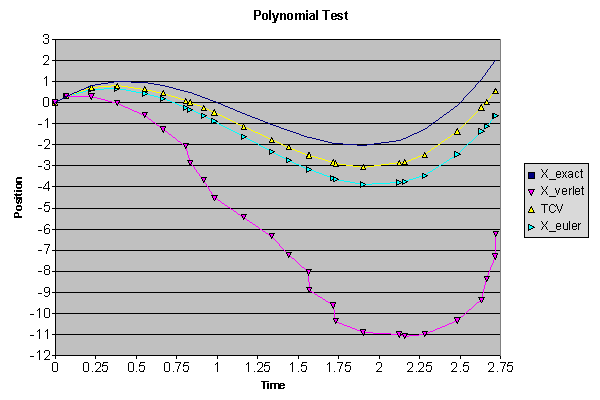
To show how the Time-Corrected Verlet behaves, a spreadsheet was set up with the TCV, the original Verlet and Euler's method, each simulating three different problems with known solutions. These are the same tests as were performed earlier, but with randomized time steps. Of course since every time step (except the first) was random, the graph looked different each time a simulation was "run". Sometimes both the original Verlet and the TCV simulations were similar, however the original Verlet always fell further away from the exact solution than the TCV version eventually. Here are some sample graphs:








Conclusion
Using the Time-Corrected form of the Verlet integration method with the proper equation for initializing the state makes the TCV integration scheme a simple, yet powerful method for doing game physics, even with changing frame rates.

It restores some of the accuracy of the method (still 4th order with constant time steps, between 2nd and 4th with changing dt), while maintaining its cheap numerical cost. I hope this helps a bit when implementing your own physics simulation code.

* Hint: remember the central difference 2[sup]nd[/sup] derivative approximation?
d[sup]2[/sup]x / dt[sup]2[/sup] = a[sub]i[/sub][sup]2[/sup]= (x[sub]i+1[/sub] - 2*x[sub]i[/sub] + x[sub]i+1[/sub]) / dt[sup]2[/sup]