If you're already familiar with the Bezier formulation of curves, then you shouldn't feel overwhelmed by the topics presented here. If you're not, read the previous article "The Practical Guide to Bezier Curves".
This article is a primer for the next article in this series. The first 2 parts are intended to set up all of the math and definitions for B-splines, and Part 3 will discuss the algorithms and shortcuts. I believe this article and its companion to be essential to understanding a very common and powerful set of curves and surfaces.
Why is this even important?
B-splines are very mathematical in nature. At some point, just like every student in a math class, you'll question why this is relevant. Before you get to that point, let me try to give a quick reason why you might want to suffer through it all. The math and algorithms presented in this series of articles form the basis of the NURBS surface technology. NURBS is highly prized by computer-aided design for its predicability, flexibility, and precision. All current 3D CAD technology relies on NURBS as the backbone for design. Everything from car bodies to airfoils to ship hulls are designed using NURBS. NURBS was also important in the development of computer graphics, and sophisticated modelers such as Blender, 3ds Max, and Maya support the use of NURBS. In addition to surfaces, NURBS curves can be used to combine several piecewise polynomial curves into one curve, a very useful operation for creating object paths, geometric entities, and so on. Although this isn't the only graphics technology in town, it's certainly a widely used one. The goal of this series is to introduce the interested game builder to this powerful set of graphical tools. Once you understand the basic math behind B-splines, I'm sure you'll be very comfortable implementing the algorithms and using them with confidence.
What is a spline?
Terminology
A spline is a smooth piecewise polynomial function. The word is derived from a thin, flexible piece of metal or wood that was placed between heavy objects on paper called "ducks" to allow draftsmen to draw curved lines. Because the ducks were placed at key points for design, the spline would interpolate points between these ducks. A mathematical spline does this same thing by interpolating curve points between control points based on equations. There are many different kinds of splines, such as Hermite splines, Catmull-Rom splines, and B-splines. The main difference between each spline is really the continuity achieved when the curves are joined. In order to appreciate this, I should define what I mean by continuity.
Continuity
Continuity between 2 curves is determined by the derivatives of the curve. If two curves share the same end point, but the value of first derivative isn't the same at the common point, then the curves are zeroth-order continuous. If the first derivatives are the same for both curves there, then it's first-order continuous. If the second derivative is the same there for both curves, then they are second-order continuous, and so on.
[If you want to get more technical, there are 2 types of continuity: parametric and geometric. Geometric continuity requires the values of the derivatives to be the same, but parametric continuity requires that the parameter values for both curves to be the same at the common point too. For example, zeroth-order geometric continuity (abbreviated \(G^0\)) requires both curves to share the same endpoint, but zeroth-order parametric continuity (abbreviated \(C^0\)) requires that both curves have the same parameter value there too (such as t=1 or something). Parametric continuity is more strict than geometric, but a general definition of \(G^n\) is that the curves can be reparameterized to be \(C^n\). Curves that are \(C^n\) with each other are automatically \(G^n\).]
Why is continuity important?
Continuity is important for several reasons. Surfaces that are \(G^1\) with each other but not \(G^2\) don't have smooth reflection lines, so a car body with \(G^1\) surfaces won't look smooth in a showroom. If you're designing a path for a railroad, for example, the railroad cars will jerk where \(G^1\) curves meet. The primary reason for CAD to be based on cubic NURBS curves or higher is that they automatically produce curves that are \(C^2\) with each other. The eye can detect discontinuities in curvature, so if we want smooth-looking curves and surfaces, we want at least \(C^2\) continuity. Because of reasons such as these, techniques have been developed to "spline" curves together to make them continuous with one another. B-splines (and NURBS by extension) are just one technique to make this happen.
Splining Bezier Curves
Are we sick of Bezier curves yet? I sure hope not! We come back to them now because splining is really about joining parametric power polynomials (say that 5x fast) and the Bezier formulation gives us just that. Let's discuss what we need to do in order to spline them together. First off, we need to remember that Bezier curves pass through the first and last control points. We can spline a series of \(G^0\) curves by simply making the last control point of one curve the first control point of the next curve. That creates an easy, albeit not smooth, curve. Let's see if we can do better. Next, we can remember that Bezier curves are tangent to the control polygon at the endpoints. That means that the curve is tangent to the line created by the last (nth) and next-to-last (n-1th) control points. If we make 2 curves \(G^0\) to each other (by making the nth point on the first curve the 1st point on the second curve), then we can force \(G^1\) continuity by making the n-1th, nth/1st, and 2nd point on the second curve all collinear. (If we wanted to, we could also force \(G^2\) continuity by controlling the position of the 2nd and n-2th control points in a similar fashion.) This is exactly how cubic Hermite splines work. The Hermite formula yields first-order continuity at given points and tangents in much the same way we forced G1 continuity above. This is a decent way to spline together points, but we only get tangent continuity. If we want anything that looks smooth, we need to do better.
The B-spline
A B-spline (or basis spline) can achieve high orders of continuity, but the tradeoff is that it's a bit harder to calculate things than with cubic Hermite splines or Bezier curves. It gets even trickier to work with when you deal with NURBS, or Non-Uniform Rational B-Splines. Because of the complexity of B-splines, people joke that "NURBS" stands for Nobody Understands Rational B-Splines. However, hopefully this and future articles can help explain them and how to use them.
Formal Definition
In my experience, there's no easy way to start talking about B-splines. There's just too much to cover and you'll discover new things as go on. As a disclaimer, I'm presenting these definitions really for completeness and to have some sort of starting point.If you have any questions about how the math or algorithms work, you will most likely need to look closer at these equations and see how things work. Everything we talk about from here on out will be based on the following equations and definitions. The formal definition of the B-spline is like the Bezier curve:
\[ C(t)=\sum_{i=0}^n P_iN_{i,p}(u) \]
As we stated above, a spline is a series of piecewise polynomials. Here, the variable p is the degree of the polynomial. As you can see from the definition, the only difference between B-splines and Bezier curves are the blending functions. For Bezier curves, the blending functions are the Bernstein polynomials. For B-splines, the blending functions are the B-spline basis functions (big surprise, right?). Before we get to them, we need to introduce the concept of a knot vector. It's a sequence of nondecreasing real numbers, and for convention it's defined as follows:
\[ U=\{u_0,\dots,u_m\};\, u_i \le u_{i+1},\, i=0,\dots,m-1 \]
Now, on to the B-spline basis functions. They are defined recursively, as follows:
\[ N_{i,0}(u) = \begin{cases} 1, & u_i \le u < u_{i+1} \\ 0, & \text{otherwise} \\ \end{cases} \\ N_{i,p}(u) = \frac{u-u_i}{u_{i+p}-u_i}\,N_{i,p-1}(u)+\frac{u_{i+p+1}-u}{u_{i+p+1}-u_{i+1}}\,N_{i+1,p-1}(u) \]
What does this mean?
I can almost hear the cries of pain, but it's really not as bad as you might think. Here's a short list of things we can tell from these equations:
- We can see that the only thing we need to compute are the basis function values for each control point to evaluate the curve.
- The degree of the polynomial doesn't determine the number of control points like in Bezier curves. Since a spline is a set of curves of the same degree, the number of control points is somewhat independent of the degree of the polynomials (remember I said "somewhat").
- The basis functions are recursive, so they're going to be a bit harder to compute than the simple evaluation we do in Bezier curves.
- Higher-order basis functions are just linear interpolations of lower order basis functions.
- The lowest order basis functions are 0th-order, which are basically step functions.
- The basis functions depend on values in the knot vector, so that means that the knot vector holds parameter value information.
Let's start exploring these curves by examining what basis functions are.
Basis Functions
Warning: Math Ahead What do I mean when I say "basis function"? Well, to understand the idea of a basis, let's start by imagining a 3D space. The standard unit vectors X, Y and Z form a basis in 3D space, meaning that every point in that 3D space can be defined as a linear combination of those unit vectors multiplied by real number coefficients.
For example, the point (2,3,4) means that we can add 2 times the unit X vector, 3 times the unit Y vector, and 4 times the unit Z vector to get to that point from the origin. We can do this kind of thing for every point in 3D space. We can use that same idea of a basis to define collections polynomials. For example, all real quadratic polynomials have the basis functions \( \{ 1, t, t^2 \} \).
That just means that if we multiply the basis functions by real numbers and add them together, we get a real quadratic polynomial, like \( f(t)=3+15t-9t^2=(3)*1+(15)*t+(-9)*t^2 \).
Now, let's talk about Bernstein polynomials. In the article Practical Guide to Bezier Surfaces, we convert the Bernstein basis polynomials into standard power polynomials (in the guide, the rightmost matrix of the Bezier curve in matrix form contains the standard power basis functions \( \{ 1,t,t^2,t^3 \} \)).
So really, Bernstein basis functions are just like power polynomials (really, they're a bit different, but you get the idea). In fact, a conversion exists between the two forms using a difference table technique (like for forward difference evaluation for Bezier curves). This means that we can express anything a power polynomial can express as a Bernstein polynomial, or in terms of the basis, as a linear combination of Bernstein basis functions. What do the Bernstein basis polynomials look like graphically? Here's a quick plot of the cubic Bernstein basis functions:
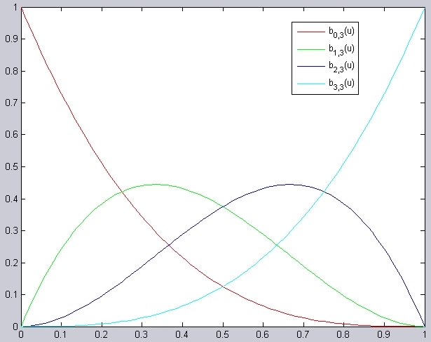
Here's a couple of things we can learn from this:
- At every value of u, the functions add up to 1 (partition of unity).
- One of the functions at either end of the graph are 1, which forces all other functions to be zero at that value. This means from the definition of Bezier curve that the curve passes through that point (endpoint interpolation)
- The graph (not each function) is symmetric about the line u=1/2.
As well, we can set up a recursive relationship with Bernstein polynomials:
\[ B_{0,0}(u) = 1 \\ B_{-1,n-1}(u) = B_{n,n-1}(u) = 0 \\ B_{i,n}(u) = 0; \, i < 0 \quad \text{or} \quad i > n \\ B_{i,n}(u) = (1-u)B_{i,n-1}(u)-uB_{i-1,n-1}(u) \]
Does this look familiar? It should! It's very similar to the B-spline basis function definition. If you're not sure that this recursive definition is correct, let me illustrate the linear and quadratic cases:
\[ \begin{align} B_{0,1}(u) &= (1-u)B_{0,0}(u)+uB_{-1,0}(u)=1-u \\ B_{1,1}(u) &= (1-u)B_{1,0}(u)+uB_{0,0}(u)=u\\ \, \\ B_{0,2}(u) &= (1-u)B_{0,1}(u)+uB_{-1,1}(u)=(1-u)^2 \\ B_{1,2}(u) &= (1-u)B_{1,1}(u)+uB_{0,1}(u)=(1-u)u+u(1-u)=2u(1-u) \\ B_{2,2}(u) &= (1-u)B_{2,1}(u)+uB_{1,1}(u)=u^2 \\ \end{align} \]
This is a good stopping point before we go on. This last bit was an attempt to tie in some of the things we'll discuss in the next article to things you've hopefully seen before, like Bezier curves and Bernstein polynomials.
Conclusion
We've discussed a lot of things in this article:
- What a spline is
- What B-splines are useful for
- The definition of continuity and why it's important
- The formal definition of a B-spline
- What a basis function is
- Properties of the Bernstein basis functions
That's a lot of information. We need all this information to understand the math behind B-splines, and in the next section, we'll start to unravel the mystery of the B-spline basis functions. Hopefully, you've been able to keep up with all this math jargon and understood it. If you haven't been able to or I just wasn't clear on some points, please leave some comments below so I can improve this article.
References
A lot of the information here was taught to me by Dr. Thomas Sederberg (associate dean at Brigham Young University, inventor of the T-splines technology, and recipient of the 2006 ACM SIGGRAPH Computer Graphics Achievement Award). The rest came from my own study of relevant literature.
Article Update Log
09 Aug 2013: Initial release