A Closer Look At Parallax Occlusion Mapping

Introduction

Parallax occlusion mapping is a technique that reduces a geometric model's complexity by encoding surface detail information in a texture. The surface information that is typically used is a height-map representation of the replaced geometry. When the model is rendered, the surface details are reconstructed in the pixel shader from the height-map texture information. I recently read through the GDC06 presentation on parallax occlusion mapping titled "Practical Parallax Occlusion Mapping for Highly Detailed Surface Rendering" by Natalya Tatarchuk of ATI Research Inc. In the presentation, an improved version of Parallax Occlusion Mapping is discussed along with possible optimizations that can be used to accelerate the technique on current and next generation hardware. Of course, after reading the presentation I had to implement the technique for myself to evaluate its performance and better understand its inner workings. This chapter attempts to present an easy to understand guide to the theory behind the algorithm as well as to provide a reference implementation of basic parallax occlusion mapping algorithm. This investigation is focused on the surface reconstruction calculations and what parameters come into play when using this technique. I have decided to implement a simple Phong lighting model. However, as you will see shortly this algorithm is very flexible and can easily be adapted to just about any lighting model that you would like to work with. In addition, a brief discussion of how to light a parallax occlusion mapped surface is also provided. The reference implementation is written in Direct3D 10 HLSL. A demonstration program is also available on the book's website that shows the algorithm in action. The demo program and the associated effect files that have been developed for this chapter are provided with it and may be used in whatever manner you desire.

This article was originally published to GameDev.net in 2006. It was revised by the original author in 2008 and published in the book Advanced Game Programming: A GameDev.net Collection, which is one of 4 books collecting both popular GameDev.net articles and new original content in print format.

Algorithm Overview

So what exactly is parallax occlusion mapping? First let's look at an image of a standard polygonal surface that we would like to apply our technique to. Let's assume that this polygonal surface is a cube, consisting of six faces with two triangles each for a total of twelve triangles. We will set the texture coordinates of each vertex such that each face of the cube will include an entire copy of the given texture. Figure 1 shows this simple polygonal surface, with normal mapping used to provide simple diffuse lighting.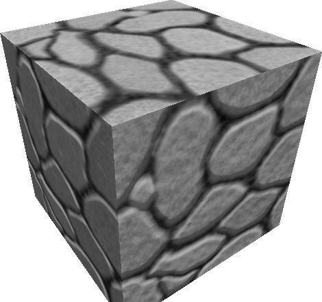 Figure 1: Flat polygonal surface 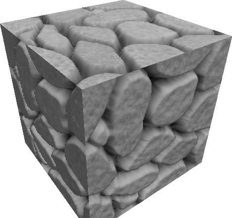The basic idea behind parallax occlusion mapping is relatively simple. For each pixel of a rendered polygonal surface, we would like to simulate a complex volumetric shape. This shape is represented by a height-map encoded into a texture that is applied to the polygonal surface. The height-map basically adds a depth component to the otherwise flat surface. Figure 2 shows the results of simulating this height-mapped surface on our sample cube. Figure 2: Flat polygonal surface approximating a volumetric shape 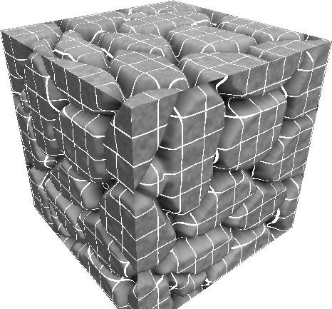The modification of the surface position can also be visualized more clearly with a grid projected onto the simulated volume. This shows the various contours that are created by modifying the surface's texture coordinates. Figure 3 demonstrates such a contour pattern. Figure 3: Gridlines projected onto the simulated surface 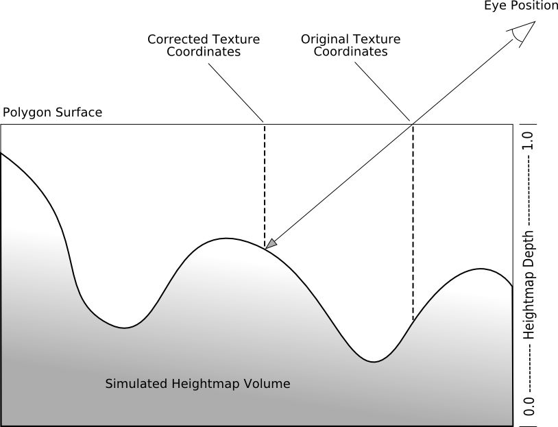We will assume that the height-map will range in value from [0.0,1.0], with a value of 1.0 representing the polygonal surface and 0.0 representing the deepest possible position of the simulated volumetric shape. To be able to correctly reconstruct the volumetric shape represented by the height map, the viewing direction must be used in conjunction with the height map data to calculate which parts of the surface would be visible at each screen pixel of the polygonal surface for the given viewing direction. This is accomplished by using a simplified ray-tracer in the pixel shader. The ray that we will be tracing is formed from the vector from the eye (or camera) location to the current rasterized pixel. Imagine this vector piercing the polygonal surface, and travelling until it hits the bottom of the virtual volume. Figure 4 shows a side profile of this intersection taking place. Figure 4: View vector intersecting the virtual volume The line segment from the polygonal surface to the bottom of the virtual volume represents the 'line of sight' for our surface. The task at hand is to figure out the first point on this segment that intersects with our height-map. That point is what would be visible to the viewer if we were to render a full geometric model of our height-map surface. Since the point of intersection between our line segment and the height-map surface represents the visible surface point at that pixel, it also implicitly describes the corrected offset texture coordinates that should be used to look up a diffuse color map, normal map, or whatever other textures you use to illuminate the surface. If this correction is carried out on all of the pixels that the polygonal surface is rendered to, then the overall effect is to reconstruct the volumetric surface - which is what we originally set out to do.

Implementing Parallax Occlusion Mapping

Now that we have a better understanding of the parallax occlusion mapping algorithm, it is time to put our newly acquired knowledge to use. First we will look at the required input texture data and how it is formatted. Then we will step through a sample implementation line by line with a thorough explanation of what is being accomplished with each section of code. The sample effect file is written in Direct3D 10 HLSL, but the implementation should apply to other shading languages as well. Before writing the parallax occlusion map effect file, let's examine the texture data that we will be using. The standard diffuse color map is provided in the RGB channels of a texture. The only additional data that is required is a height-map of the volumetric surface that we are trying to simulate. In this example, the height data will be stored in the alpha channel of a normal map where a value of 0 (shown in black) corresponds to the deepest point, and a value of 1 (shown in white) corresponds to the original polygonal surface. Figure 5 shows the color texture, alpha channel height-map, and the normal map that it will be coupled with.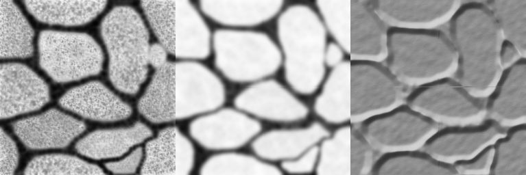 Figure 5: Sample color map, normal map, and height map. It is worth noting that the normal map is not required to implement this technique - it is used here for simplified shading purposes, but is not required to perform the parallax occlusion mapping technique. With a clear picture of the texture data that will be used, we will now look into the vertex shader to see how we set up the parallax occlusion mapping pixel shader. The first step in the vertex shader is to calculate the vector from the eye (or camera) position to the vertex. This is done by transforming the vertex position to world space, and then subtracting its position from the eye position. The world space vertex position is also used to find the eye vector and the light direction vector. float3 P = mul( float4( IN.position, 1 ), mW ).xyz; float3 N = IN.normal; float3 E = P - EyePosition.xyz; float3 L = LightPosition.xyz - P; Next, we must transform the eye vector, light direction vector, and the vertex normal to tangent space. The transformation matrix that we will use is based on the vertex normal, binormal, and tangent vectors. float3x3 tangentToWorldSpace; tangentToWorldSpace[0] = mul( normalize( IN.tangent ), mW ); tangentToWorldSpace[1] = mul( normalize( IN.binormal ), mW ); tangentToWorldSpace[2] = mul( normalize( IN.normal ), mW ); Each of these vectors is transformed to world space, and are then used to form the basis of the rotation matrix for converting a vector from tangent to world space. Since this is a rotation only matrix, then if we transpose the matrix it becomes its own inverse. This produces the world to tangent space rotation matrix that we need. float3x3 worldToTangentSpace = transpose(tangentToWorldSpace); Now the output vertex position and the output texture coordinates are trivially calculated. OUT.position = mul( float4(IN.position, 1), mWVP ); OUT.texcoord = IN.texcoord; And finally, we use the world to tangent space rotation matrix to transform the eye vector, light direction vector, and the vertex normal to tangent space. OUT.eye = mul( E, worldToTangentSpace ); OUT.normal = mul( N, worldToTangentSpace ); OUT.light = mul( L, worldToTangentSpace ); That is all there is for the vertex shader. Now we move on to the pixel shader, which contains the actual parallax occlusion mapping code. The first calculation in the pixel shader is to determine the maximum parallax offset length that can be allowed. This is calculated in the same way that standard parallax mapping does it. The maximum parallax offset is a function of the depth of the surface (specified here as fHeightMapScale), as well as the orientation of the eye vector to the surface. For a further explanation see "Parallax Mapping with Offset Limiting: A Per-Pixel Approximation of Uneven Surfaces" by Terry Welsh. float fParallaxLimit = -length( IN.eye.xy ) / IN.eye.z; fParallaxLimit *= fHeightMapScale; Next we calculate the direction of the offset vector. This is essentially a two dimensional vector that exists in the xy-plane of the tangent space. This must be the case, since the texture coordinates are on the polygon surface with z = 0 (in tangent space) for the entire surface. The calculation is performed by finding the normalized vector in the direction of offset, which is essentially the vector formed from the x and y components of the eye vector. This direction is then scaled by the maximum parallax offset calculated in the previous step. float2 vOffsetDir = normalize( IN.eye.xy ); float2 vMaxOffset = vOffsetDir * fParallaxLimit; Then the number of samples is determined by lerping between a user specified minimum and maximum number of samples. int nNumSamples = (int)lerp( nMaxSamples, nMinSamples, dot( E, N ) ); Since the total height of the simulated volume is 1.0, then starting from the top of the volume where the eye vector intersects the polygon surface provides an initial height 1.0. As we take each additional sample, the height of the vector at the point that we are sampling is reduced by the reciprocal of the number of samples. This effectively splits up the 0.0-1.0 height into n chunks where n is the number of samples. This means that the larger the number of samples, the finer the height variation we can detect in the height map. float fStepSize = 1.0 / (float)nNumSamples; Since we would like to use dynamic branching in our sampling algorithm, we must not use any instructions that require gradient calculations within the dynamic loop section. This means that for our texture sampling we must use SampleGrad instruction instead of a plain Sample instruction. In order to use SampleGrad, we must manually calculate the texture coordinate gradients in screen space outside of the dynamic loop. This is done with the intrinsic ddx and ddy instructions. float2 dx = ddx( IN.texcoord ); float2 dy = ddy( IN.texcoord ); Now we initialize the required variables for our dynamic loop. The purpose of the loop is to find the intersection of the eye vector with the height-map as efficiently as possible. So when we find the intersection, we want to terminate the loop early and save any unnecessary texture sampling efforts. We start with a comparison height of 1.0 (corresponding to the top of the virtual volume), initial parallax offset vectors of (0,0), and starting at the 0th sample. float fCurrRayHeight = 1.0; float2 vCurrOffset = float2( 0, 0 ); float2 vLastOffset = float2( 0, 0 ); float fLastSampledHeight = 1; float fCurrSampledHeight = 1; int nCurrSample = 0; Next is the dynamic loop itself. For each iteration of the loop, we sample the texture coordinates along our parallax offset vector. For each of these samples, we compare the alpha component value to the current height of the eye vector. If the eye vector has a larger height value than the height-map, then we have not found the intersection yet. If the eye vector has a smaller height value than the height-map, then we have found the intersection and it exists somewhere between the current sample and the previous sample. while ( nCurrSample < nNumSamples ) { fCurrSampledHeight = NormalHeightMap.SampleGrad( LinearSampler, IN.texcoord + vCurrOffset, dx, dy ).a; if ( fCurrSampledHeight > fCurrRayHeight ) { float delta1 = fCurrSampledHeight - fCurrRayHeight; float delta2 = ( fCurrRayHeight + fStepSize ) - fLastSampledHeight; float ratio = delta1/(delta1+delta2); vCurrOffset = (ratio) * vLastOffset + (1.0-ratio) * vCurrOffset; nCurrSample = nNumSamples + 1; } else { nCurrSample++; fCurrRayHeight -= fStepSize; vLastOffset = vCurrOffset; vCurrOffset += fStepSize * vMaxOffset; fLastSampledHeight = fCurrSampledHeight; } } Once the pre- and post-intersection samples have been found, we solve for the linearly approximated intersection point between the last two samples. This is done by finding the intersection of the two line segments formed between the last two samples and the last two eye vector heights. Then a final sample is taken at this interpolated final offset, which is considered the final intersection point. float2 vFinalCoords = IN.texcoord + vCurrOffset; float4 vFinalNormal = NormalHeightMap.Sample( LinearSampler, vFinalCoords ); //.a; float4 vFinalColor = ColorMap.Sample( LinearSampler, vFinalCoords ); // Expand the final normal vector from [0,1] to [-1,1] range. vFinalNormal = vFinalNormal * 2.0f - 1.0f; Now all that is left is to illuminate the pixel based on these new offset texture coordinates. In our example here, we utilize the normal map normal vector to calculate a diffuse and ambient lighting term. Since the height map is stored in the alpha channel of the normal map, we already have the normal map sample available to us. These diffuse and ambient terms are then used to modulate the color map sample from our final intersection point. In the place of this simple lighting model, you could use the offset texture coordinates to sample a normal map, gloss map or whatever other textures are needed to implement your favorite lighting model. float3 vAmbient = vFinalColor.rgb * 0.1f; float3 vDiffuse = vFinalColor.rgb * max( 0.0f, dot( L, vFinalNormal.xyz ) ) * 0.5f; vFinalColor.rgb = vAmbient + vDiffuse; OUT.color = vFinalColor; Now that we have seen parallax occlusion mapping at work, let's consider some of the parameters that are important to the visual quality and the speed of the algorithm.

Algorithm Metrics

The algorithm as presented in the demonstration program's effect file runs at faster than the 60 Hz refresh rate of my laptop with an Geforce 8600M GT at a screen resolution of 640x480 with the minimum and maximum number of samples set to 4 and 20, respectively. Of course this will vary by machine, but it will serve as a good metric to base performance characteristics on since we know that the algorithm is pixel shader bound. The algorithm is implemented using shader model 3.0 and later constructs - specifically it uses dynamic branching in the pixel shader to reduce the number of unnecessary loops after the surface intersection has already been found. Thus relatively modern hardware is needed to run this effect in hardware. Even with newer hardware, the algorithm is pixel shader intensive. Each iteration of the dynamic loop that does not find the intersection requires a texture lookup along with all of the ALU and logical instructions used to test if the intersection has occurred. Considering that the sample images were generated with a minimum sample count of 4 and a maximum sample count of 20, you can see that the number of times that the loop is performed to find the intersection is going to be the most performance critical parameter. With this in mind, we should develop some methodology for determining how many samples are required for an acceptable image quality. Figure 6 compares images generated with 20 and then 6 maximum samples respectively.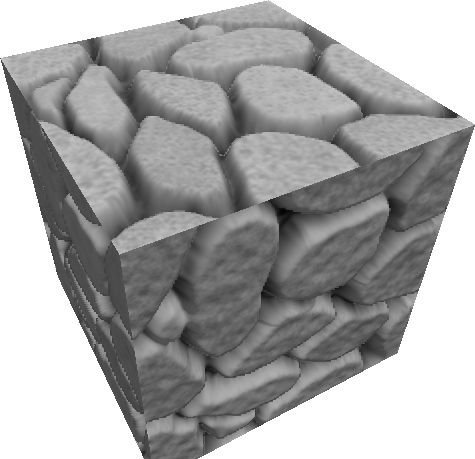 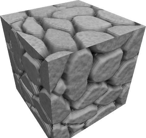Figure 6: A 20-sample maximum image (top) and a 10-sample maximum image (bottom)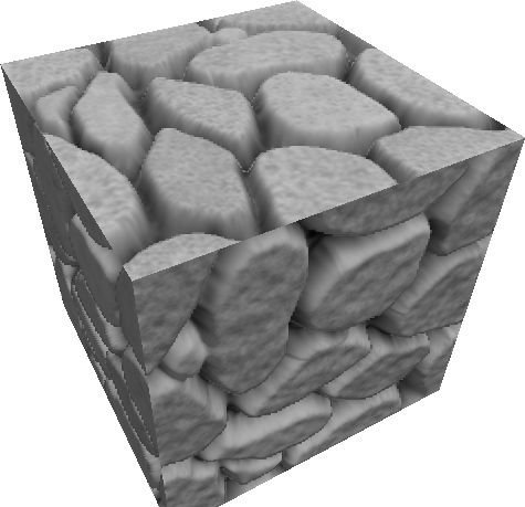 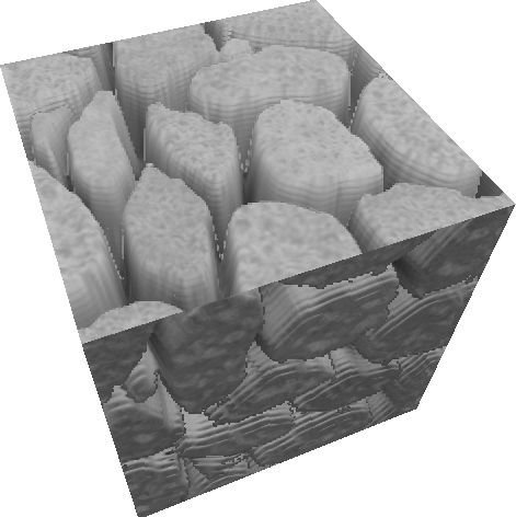As you can see, there are aliasing artifacts along the left hand side of the 6-sample image where the height map makes any sharp transitions. Even so, the parts of the image that do not have such a sharp transition still have acceptable image quality. Thus, if you will be using low frequency height map textures, you may be able to significantly reduce your sampling rate without any visual impact. It should also be noted that the aliasing is more severe when the original polygon surface normal is closer to perpendicular to the viewing direction. This allows you to adjust the number of samples based on the average viewing angle that will be used for the object being rendered. For example, if a wall is being rendered that will always be some distance from the viewer then a much lower sampling rate can be used then if the viewer can stand next to the wall and look straight down its entire length. Another very important parameter that must be taken into consideration is the height-map scale, named fHeightMapScale in the sample effect file. If you imagine a 1-meter by 1-meter square (in world space coordinates), then the height-map scale is how deep of a simulated volume we are trying to represent. For example, if the height-map scale is 0.04, then our 1x1 square would have a potential depth of 0.04 meters. Figure 7 shows two images generated with a scale height of 0.1 and 0.4 with the same sampling rates (20 samples maximum). Figure 6: A 0.1 height map scale image (top) and a 0.4 height map scale image (bottom) 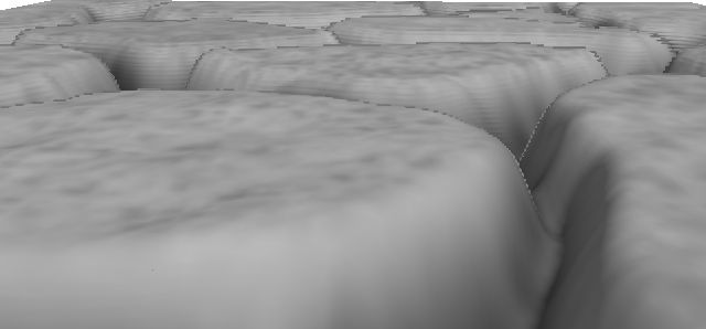It is easy to see the dramatic amount of occlusion caused by the increased scale height, making the contours appear much deeper than in the original image. Also notice toward the bottom of the image that the aliasing artifacts are back - even though the sampling rates are the same. With this in mind, you can see that the height scale also determines how 'sharp' the features are with respect to the eye vector. The taller the features are, the harder they will be to detect intersections with the eye vector. This means that we would need more samples per pixel to obtain similar image quality if the height scale is larger. So a smaller height scale is "a good thing". In addition, let's look deeper into how the algorithm will react when viewing polygonal surfaces nearly edge on. Our current algorithm uses a maximum of 20 samples to determine where the intersections are. This is already a significant number of instructions to run, but the image quality is going to be low when viewed from an oblique angle. Here's why. If your height map is 256x256, and you view our 1m x 1m square from the edge on, then in the worst case you can potentially have a single screen pixel be required to test 256 texels for intersections before it finds the surface of the height map. We would need ~12 times more samples than our maximum sampling rate to get an accurate intersection point! Figure 8 shows an edge on image generated with 50 samples and 0.1 height-map scale. Figure 7: A 60-sample 0.04 height-map scale image from an oblique angle Mip-mapping would help this situation by using a smaller dimension version of the texture when at extreme angles like this, but by each level of mip-map reducing the resolution of the height-map it could potentially introduce additional artifacts. Care must be taken to restrict the number of situations where an object would be viewed edge on, or to switch to a constant time algorithm like bump mapping at sharp angles. The ideal sampling situation would be to have one sample for each texel that the eye vector could possibly pass through during the intersection test. So a straight on view would only require a single sample, and an edge on view would require as many samples as there are texels in line with the pixel (up to a maximum of the number of texels per edge). This is actually information that is already available to us in the pixel shader. Our maximum parallax offset vector length, named fParallaxLimit in the pixel shader, is a measure of the possible intersection test travel in texture units (the xy-plane in tangent space). It is shorter for straight on views and longer for edge on views, which is what we want to base our number of samples on anyways. For example, if the parallax limit is 0.5 then a 256x256 height-map should sample, at most, 128 texels. This sampling method will provide the best quality results, but will run slower due to the larger number of iterations. Whatever sampling algorithm is used, it should be chosen to provide the minimum number of samples that provides acceptable image quality. Another consideration should be given to how large an object is going to appear on screen. If you are using parallax occlusion mapping on an object that takes up 80% of the frame buffer's pixels, then it will be much more prohibitive than an object that is going to take 20% of the screen. So even if your target hardware can't handle full screen parallax occlusion mapping, you could still use it for smaller objects.

Conclusion

I decided to write this article to provide some insight into the parallax occlusion mapping algorithm. Hopefully it is easy to understand and will provide some help in implementing the basic algorithm in addition to giving some hints about the performance vs. quality tradeoff that must be made. I think that the next advance in this algorithm is probably going to be making it more efficient, most likely with either a better sampling rate metric, or with a data structure built into the texture data to accelerate the searching process. If you have questions or comments on this document, please feel free to contact me as 'Jason Z' on the GameDev.net forums or you could also PM me on GameDev.net.