Despite how important of a topic good importance sampling is in the area of global illumination, it's usually left out of all common-English conversations and tutorials about path tracing (with the exception of the Lambertian case, which is a good introduction to importance sampling). If you want to get into microfacet importance sampling, multiple importance sampling, or even, God forbid, Metropolis light transport, you're on your own. And, probably for a good reason. At some point in a path tracing project, you WILL have to butt heads with the math. And believe me, the head that the math rears is ugly. Beautiful in design, but large and ugly all the same.

I'm going to try to correct that, at least for microfacet importance sampling. Present just enough math to get the point across what *needs* to be understood to implement everything correctly, with minimal pain.

Choosing the Microfacet Terms

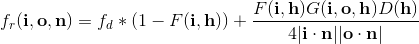
The Cook-Torrance Microfacet BRDF for specular reflections comes in the form

, where F is the Fresnel term, D is the microfacet distribution term, and G is the microfacet shadowing term.

This is great and all, as it allows you to basically stop and swap different terms in as much as you want. Realtime graphics use that property to be able to simplify a BRDF into something pretty but efficient, by mixing and matching models with terms that cancel out.

However, there is danger in this though. Choosing terms purely because they are less complex, and therefore more efficient, can lead to completely wrong results. As a case in point, let me show the difference between the implicit Smith G and the Beckmann with Smith G. For reference:

For future reference, the Beckmann G1 listed is an approximation to the actual Beckmann shadowing term. The alpha_b is a tunable parameter that controls the roughness of the material. I usually just set that term to the Cook-Torrance roughness value.

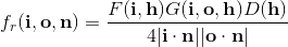
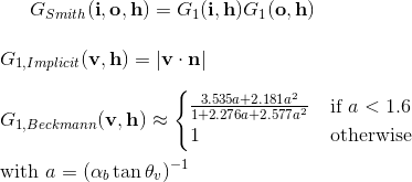
These are the results, after importance sampling for 500 samples:

Top: Implicit G1, roughness 0.05, 500 samples of importance sampling
Bottom: Beckmann G1, roughness 0.05, 500 samples of importance sampling

As you can see, the Implicit G suffers greatly for its simplicity. While it calculates color noticeably faster, it does so by ignoring the cases that need extra work to represent, like really low roughness values. It approximates the mid-range fairly well, but in doing so butchers the tails. So take this example to heart: for a path tracer, don't be afraid to sacrifice a little speed for correct color, especially because people use pathtracers because they're willing to wait for good images.

So. What terms should be chosen? Well, my personal favorite $$ D $$ and $$ G $$ are the Beckmann ones, so this post is going to be based off of those. A more complete description of the *whys* of all of this can be found [here](https://www.cs.cornell.edu/~srm/publications/EGSR07-btdf.pdf), but as titled, this is the "For Dummies" version, and re-stating everything found there would be a massive waste of time.

The Fresnel term is taken from Cook-Torrance:

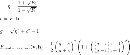
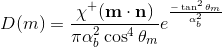
The Distribution term is from Beckmann:

The Geometry term is a little trickier. It involves the erf(x) function, which can be very expensive to calculate. There's an approximation of it, though, that's very good, shown again here:

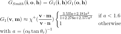
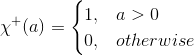
The only things left to clarify is alpha_b term, which is just the roughness of the material, and the chi^+ function, which enforces positivity:

Importance Sampling

So to importance sample the microfacet model shown above involves a lot of integrals. So many that I'll probably end up getting LaTex-pinky from typing all the brackets. So I'm just going to give the short version.

Because it'd be damn near impossible to try to importance sample the entire microfacet model, with all of its terms together, the strategy is to importance sample the distribution term to get a microfacet normal, and then transform everything from all vectors relative to the normal to relative to the origin.

Given 2 uniform random variables, zeta1 and zeta2, generate a microfacet normal with the angles (relative to the surface normal):

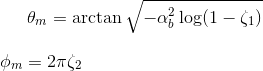
Note how the phi_m term is can spin freely around the normal. This is the power that sampling only the D function has. It follows, then, that by reversing the age-old vector-reflectance equation, you get the outbound (or inbound, or whatever) light ray:

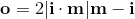
Now all that's left to do, with the exception of a few caveats that I will get to in a minute, is to define the probability distribution function for this setup:

There! That's all that's needed! If all you want to do is render really shiny metals, at least. However, there's some unfinished business we have to attend to concerning what to do with the un-reflected light, the amount that the Fresnel term takes away. First, though, let's look at some images.

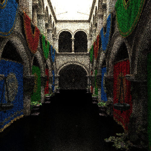
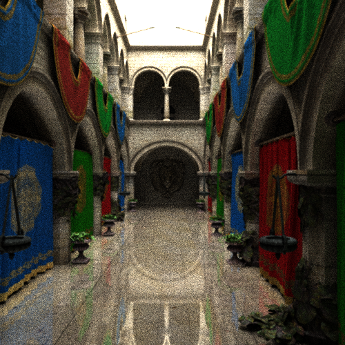
Intermediate Results

[Above: Sponza atrium with a floor with Cook-Torrance roughness of 0.001, 500 samples per pixel]

What's impressive about the above image is that that isn't a mirror BRDF. It's the microfacet BRDF described above, importance sampled. This amount of image clarity for a floor with a roughness that small, and at only 500 samples, is something that would have only been achieved with a special-case in the code for materials like that. However, with importance sampling, you get it all for free!

Extending it With Lambertian Diffuse

The Cook-Torrance BRDF is really nice and all, but it's only a specular BRDF after all. We need to fuse it with a Lambertian BRDF to finish everything up nicely. The form the BRDF takes after the fuse is:

This makes a lot of sense too. A Fresnel Term describes how the ratio between reflected and transmitted signals, and a diffuse reflection is just a really short-range refraction.

Now there's an issue, and it's a big one. The density function generated above describes the distribution of outbound rays based off of the D microfacet distribution. To convert between a microfacet distribution and an outbound ray distribution, it undergoes a change of base via a Jacobian. Now that Jacobian is analytically derived from the microfacet BRDF definition itself, so to integrate the diffuse term into it (a term which has no microfacets but still changes the shape of the BRDF drastically) it'd have to be re-calculated.

And this is a re-occurring problem. There are papers describing every way to couple this with that. Some of them are about coupling matte diffuse with microfacet specular, some describe how to couple transmissive plus specular, some specular with specular. And at the end of the day, these are all specialized cases of different material properties coexisting on a surface. Until it's taken care of, the problem of mixing and matching BRDFs will never go away. I don't know how other path tracers deal with this issue, but I won't stand for it.

For my path tracer, I chose to go the way that Arnold does, by using the idea of infinitesimal layers of materials. Each layer of the material can, by using the Fresnel function we already have, reflect an amount of light, and then transmit the rest down to the next layer down. This will happen for every layer down until it hits the final layer: either a diffuse or transmission layer, which will use the rest of the remaining energy. Thus, the problem of coupling BRDFs was solved by thinking about the problem a little differently.

If you think about it, the above algorithm can be simplified using Russian Roulette, and so the final algorithm becomes something like this:[code=:0]Generate random number r1for each layer in material: determine the new half-vector (or microfacet normal) f = Fresnel function using that half-vector if (r1 > f): r1 -= f continue calculate outbound ray generate BRDF for current layer and inbound and outbound rays generate pdf for outbound ray sample and accumulate as normal break

The only thing left to do is get rid of the Fresnel term from the microfacet BRDF and the (1 - F) from in front of the Lambertian term: it won't be of any more use to us right there, as that calculation is handled implicitly now. That function now serves as a Russian Roulette mechanism to switch between layers, and is no longer needed to scale the energy of the microfacet BRDF, as the D and G term are perfectly capable of doing exactly that on their own.

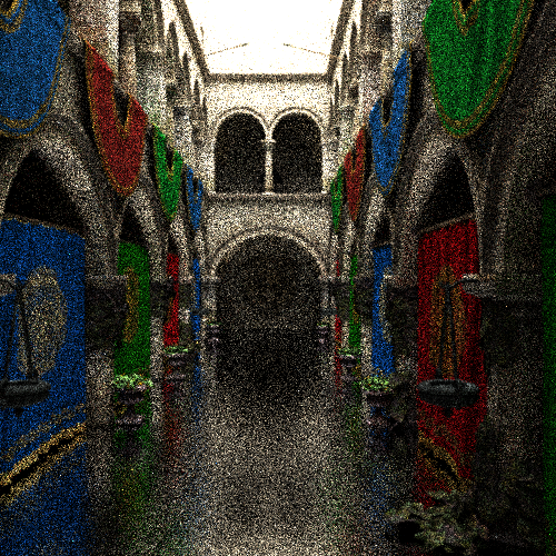
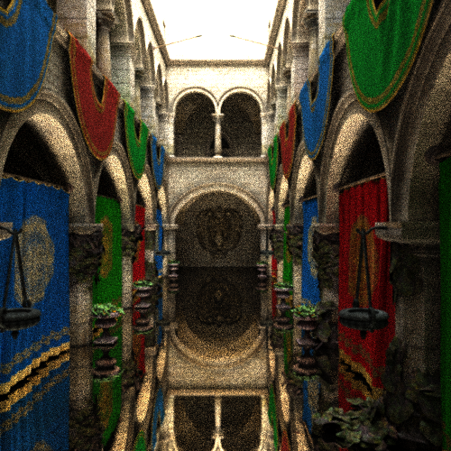
One more pic to show it in action:

[Above: Floor with layered specular and diffuse. 500 samples per pixel]

That concludes my write-up of Microfacet Importance Sampling: For Dummies edition. With luck, hopefully implementing it will be as enjoyable for you as it was for me. Happy rendering, and may your dividends be forever non-zero! :D