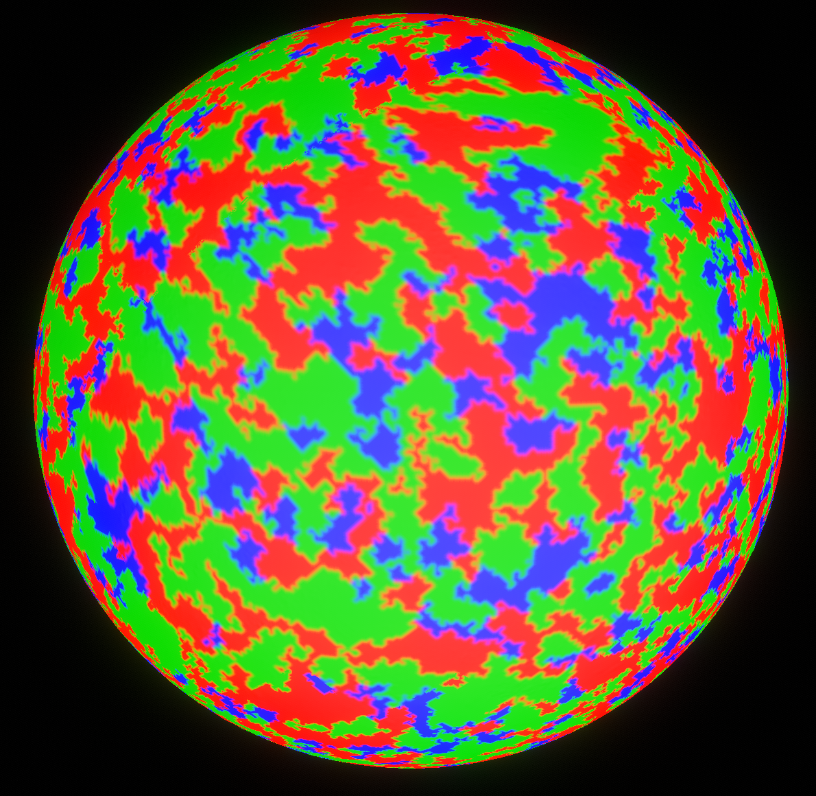
In this post I will share a new technique I developed for interpolation/upsampling of data. This method is able to produce interesting looking results such as this from very low resolution input:

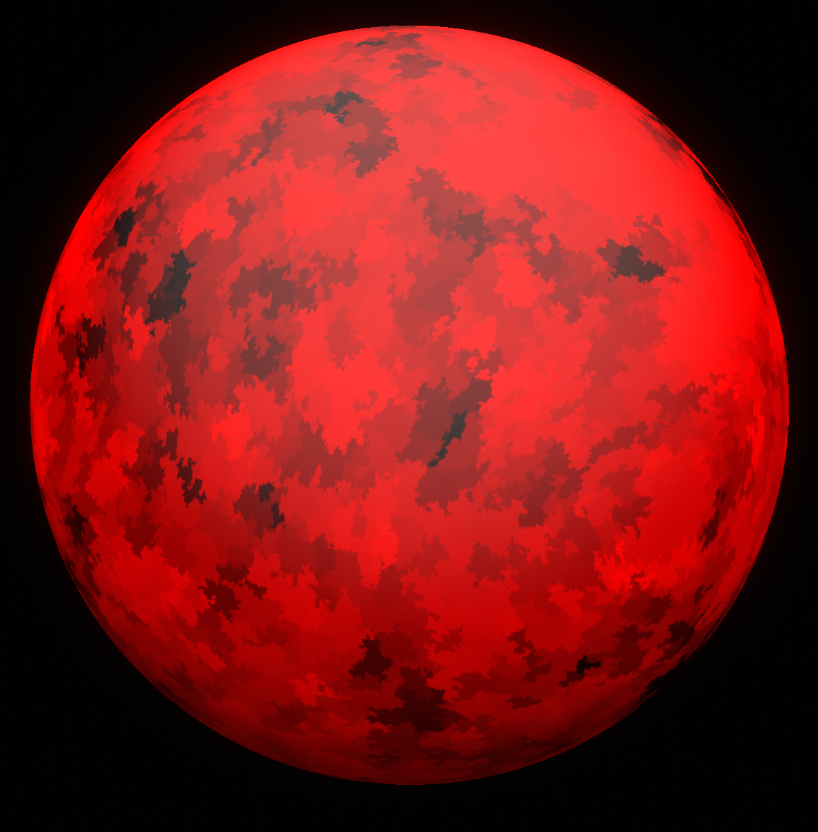
This image was generated by applying the interpolation technique recursively to random white noise data on the surface of a sphere at 33x33 resolution per cube face. You can see that it generates discrete regions which have a fractal border. It is possible to zoom into this fractal infinitely, with more border detail added as you zoom in.

Background

When doing procedural generation, it is often useful to be able to repeatedly upscale an image (e.g. height map, noise field, etc.), so that detail can be added on top of lower-resolution LODs. Most interpolation techniques focus on how to do this smoothly by doing bilinear, biquadratic, or bicubic interpolation, for example. These methods produce an output that is very smooth and useful for smooth things like terrain. However, often we want to preserve harder edges when upscaling, especially if the data to be interpolated is stored as integers, where mixing adjacent values would produce undesired results. For instance, we might want to upscale the material IDs or biome type of the terrain when zooming in to denser LOD.

A common suggestion for generating discrete regions is to use Voronoi cells. However, these are generally too regular when generated using efficient grid-based methods. Every region would have approximately the same size and shape. The method presented here is an alternative to Voronoi that is both much more efficient, easier to implement, and produces more natural-looking results.

The main goal of the interpolation technique described in this post is to do interpolation without mixing values, while producing an output that looks organic and natural. In this post I only consider upscaling by a factor of 2.

Nearest Neighbor Interpolation

The most basic kind of interpolation that fulfills the hard-edges requirement is to do nearest-neighbor interpolation. With an upscale factor of 2x, this method effectively would double each pixel, producing blocky-looking results. The output would look like the image was magnified without adding any detail. When this method is applied recursively, the blockiness persists.

This method can be used to generate terrains that look like “death star” topography, with numerous rectangular terraces. However, this is not very useful in practice, since it looks very artificial. This led me to develop a more capable method.

Dithered Nearest Neighbor Interpolation

To avoid the problems of standard nearest neighbor, I developed a method I call “dithered nearest neighbor” interpolation. The main idea is to randomly choose the values of the new pixels based on white noise values. Consider a 2x2 square of pixels which we want to upscale to 3x3 pixels:

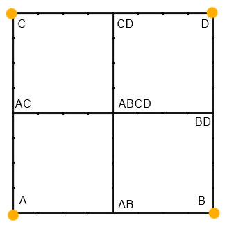
Here I have labeled the original 4 vertices (A, B, C, D), and the new vertices to be generated (AB, AC, BD, CD, ABCD). The input to the algorithm is just the values at vertices A, B, C, D. For all 9 vertices (both old and new), we generate a random noise value (noise can be float or integer). Then, using those noise values we can choose which of the A, B, C, D values to use for each output pixel according to the following rules:

• A - same as input
• B - same as input
• C - same as input
• D - same as input
• AB - choose A or B based on whether Noise(AB) is closer to Noise(A) or Noise(B).
• AC - choose A or C based on whether Noise(AC) is closer to Noise(A) or Noise(C).
• BD - choose B or D based on whether Noise(BD) is closer to Noise(B) or Noise(D).
• CD - choose C or D based on whether Noise(CD) is closer to Noise(C) or Noise(D).
• ABCD - choose A, B, C, or D, based on whether Noise(ABCD) is closer to Noise(A), Noise(B), Noise(C), or Noise(D).

You might wonder why we don't just choose either A or B based on if Noise(AB) < 0.5, since that would be simpler than comparing Noise(AB) to Noise(A) and Noise(B) then choosing the closer one. The reason for the presented method is that it is rotationally-invariant, while the alternatives would produce different results depending on if the image was rotated. This is an important property if you want to apply this method to data on a sphere and not produce any seams between adjacent cube faces. For instance, the Y+ and Z- faces on a cube map share an edge with a 180 degree rotation, and without rotational invariance, there would be a seam produced at that edge. (I had this bug for months)

Using the presented rules, we can upscale a single 2x2 pixel quad to a 3x3 area. It's not difficult to extend this to upscale images of any size by a factor of 2. That can be done by independently processing each 2x2 quad in the image, and only computing the AB, AC, and ABCD values, since the others will be calculated by the neighboring 2x2 areas. There is a special case for the last row and column (the CD and BD cases), which needs to be handled differently.

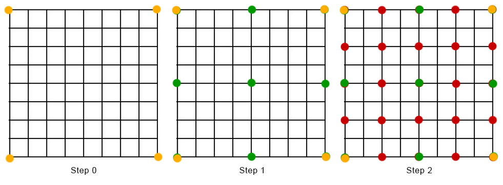
We can extend this method to produce more interesting results by applying these rules recursively, as illustrated by the following image. First, the green vertices are interpolated, then red, then finally the uncolored vertices.

The results of applying this method recursively to a 4x4 input data are shown below.

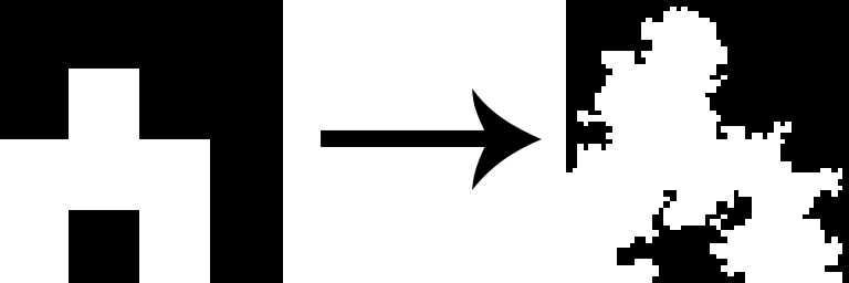
Here we have a very simple shape that has been turned into something very interesting with fractal borders, simply by applying this interpolation method several times. Detail is continually added to the borders as the image is enlarged more.

Smoothing It Out

While this is already quite a useful approach for enlarging images, in many cases we want something between dithered nearest neighbor (DNN) and another smoother interpolation method. For instance, we might want to use DNN to interpolate the biomes on the surface of a planet so that they have interesting borders. However, we don't want instant transitions between adjacent biomes. Ideally we would want a smooth transition to occur beyond a certain scale (e.g. below 10km per pixel).

To fix this, we can combine the DNN method with another smoother method by switching between the methods at a certain level of detail. DNN is used at macro scales (e.g. down to 1 heightmap pixel = 10km), while biquadratic interpolation can be used for finer LODs. This produces more natural results with floating point data that can be interpolated. The following image shows the same example as above but with the addition of biquadratic interpolation past a certain scale.

This retains the fractal shape of the basic DNN method, but smooths it out at a certain point.

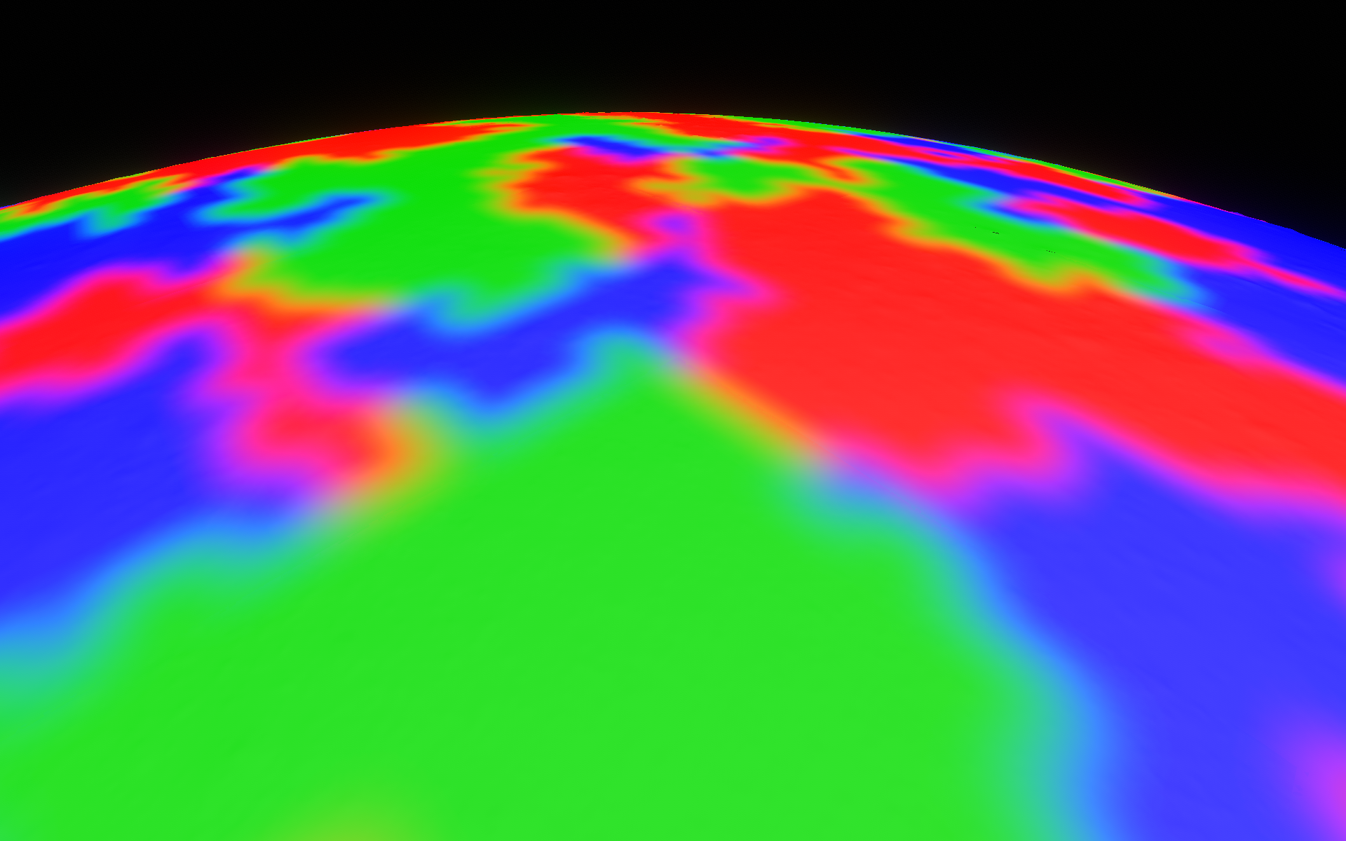
The next few images show how this looks when applied to a planet. There are 3 different “biome” types on this planet, indicated by red, green, and blue colors. When zoomed in, you can see that the borders are smooth, but also with some fractal detail.

Example: Planet Materials

This final image shows how this can look when it is used to generate the materials on the surface of a planet. There are about possible 16 materials here, generated in 4 planet-wide regions where each region has different probabilities for the materials to be present. DNN-based noise is used to sample the material that is present at each pixel.

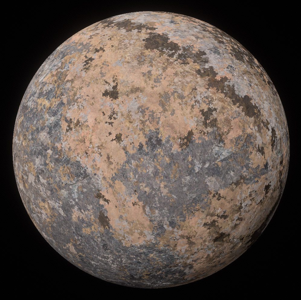
If you look closely, you can see a seam in the middle-right of the image. This is the result that you get if the DNN is not rotationally invariant. This seam has since been fixed by using the rotationally-invariant method.